Week 7 - Simulation of a 1D Super-sonic nozzle flow simulation using Macormack Method

Theory:

A nozzle is a device used to modify a fluid flow's characteristics as it exits (or enters) a closed chamber or conduit, with the goal of increasing velocity in particular. When controlling, directing, or changing the flow of a fluid, a nozzle is frequently a pipe or tube having a changeable cross sectional area (liquid or gas). Nozzles are frequently used to control the flow, speed, direction, mass, shape, and/or pressure of the stream that exits them.

There are several nozzle varieties. In this project, we use a divergent-convergent nozzle, however. This nozzle allows for the production of a supersonic stream at low input speeds. The Mach number should then increase from Ma=0 at the inlet to Ma>1 as you get closer to the exit. It follows naturally that the nozzle must diverge in the supersonic area and converge in the subsonic zone. One such nozzle is the convergent-divergent nozzle.

Convergent nozzles manage sonic and subsonic flows. These are also tools for measuring and regulating flow.
Convergence-divergence nozzles are used for supersonic flows. Convergent-divergent passages in compressor and turbine blade rows are very difficult to accomplish.
In this project, the convergent-divergent nozzle is taken into account, and the 1D supersonic nozzle flow equations are solved using the Macormack Method algorithm.

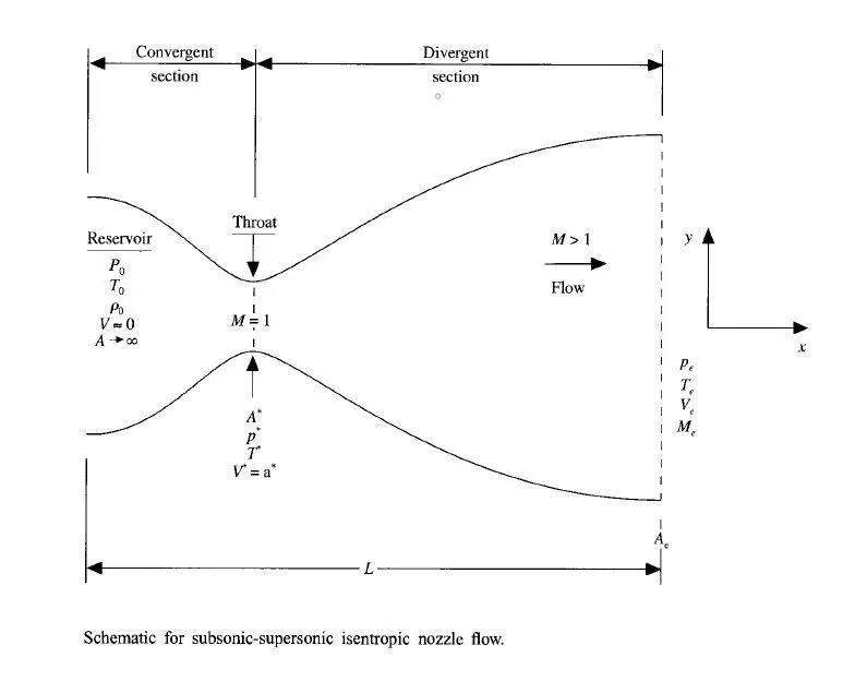
Here we consider the steady isentropic flow via a convergent-divergent nozzle. The flow enters the nozzle at the entrance at the pressure and temperature of the reservoir, denoted by the letters Pe,Te,VeandMe">Po and Pe,Te,VeandMe">To, respectively.
The extraordinarily low velocity (V = 0) is caused by the reserve's enormous cross-sectional area (A = infinity). Thus, the standstill values are Pe,Te,VeandMe">Po and Pe,Te,VeandMe">To, or total pressure and total temperature. The exit pressure, temperature, velocity, and Mach number are displayed at the nozzle exit, where the flow expands isentropically to supersonic speeds by Pe,Te,VeandMe">Pe,Te,VeandMePe,Te,VeandMe .

In the convergent region of the nozzle, the flow is locally subsonic, sonic at the throat, and supersonic in the divergent section. The local velocity at the throat is equal to the local speed of sound because of the sonic flow (M=1) at this position. We use the symbols P*, T*, V* (which is equal to V* = a* (speed of sound)), and A to signify the pressure, temperature, velocity, and area.

Step-1 - Governing equations

For Non Conservative :-

Continuity Equation

Momentum Equation

Energy Equation

For Conservative :-

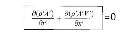
Continuity Equation

Momentum Equation

Energy Equation

MacCormack Method:

This approach is utilised to solve the governing equations of quasi 1D supersonic nozzle flow as opposed to the differencing procedures that we previously investigated. A second order precise explicit finite difference approach in both time and space is the Maccormack method. In computational fluid dynamics, the MacCormack approach is a well-liked discretization technique for the numerical solution of hyperbolic partial differential equations. The code that follows will demonstrate how this method just needs two phases to work effectively: a prediction step and a corrector step.

The predictor step:

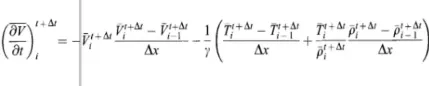
In the predictor phase, the geographic terms on the right side of the equation are switched out for forward differences. The RHS of the equation may be determined since all of the variable values are for time-step "t". The time marching solution is then applied to the computation of the variable's value on the LHS to determine the value of the variable at each grid point for time-step "t+dt."

(∂v∂t)=(∂ρ∂x)">

(∂v∂t)=(∂ρ∂x)">Corrector Step:

The correction step replaces the spatial term on the right with the backward difference. The values ​​of the variables are derived from the prediction step of the 't+dt' time step of RHS. The corrected time derivative is then calculated. Then, using the predicted and corrected values ​​of the time derivative, the average time derivative, which gives the value of the variable at a particular point in a particular time step is calculated. The properties of fluids as they pass through a converging-diverging nozzle are the focus of this project. The same steps are repeated until the values ​​of the variables are obtained for all grid points for a fixed number of time steps. Fluid properties of conservative and non-conservative flows are studied. There are differences between conservative and non-conservative numerical methods, but they are mathematically equivalent. You can accurately transform one shape into another.

Average :

Governing equations for Quasi 1-D Supersonic nozzle flow

The governing contunity,momentum and energy equations for Quasi 1D steady icentropic flow is given by

Contunity Equation:

ρ1V1A1=ρ2V2A2">ρ1V1A1=ρ2V2A2ρ1V1A1=ρ2V2A2

Momentum Equation:

ρ1A1+ρ1V12+∫pdV=p2A2+ρ1V22"> ρ1A1+ρ1V21+∫pdV=p2A2+ρ1V22ρ1A1+ρ1V12+∫pdV=p2A2+ρ1V22

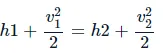
Energy Equation:

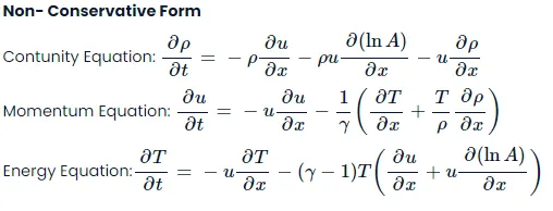
The values of each variable are not dimensional. Following the Maccormack method's solution of these equations, the steady-state values of all variables, including temperature, velocity, and density, are discovered. These variables are used to calculate the Mach number and pressure.

Time step :

In order for the solution to be stable, the concept of Courant flow number was introduced in previous projects. For a linear Hyperbolic equation, the value of CFL<1 will give a stable solution

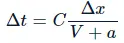CFL=0.5

where an is the local speed of sound, V is the local flow velocity at a place, and C is the Courant number. All grid points' values for dt are computed, and the simulation will use the value with the lowest value.

Boundary Conditions-

At the inlet:

Velocity at the inlet is changing with time, while the density and temperature are constant with respect to time.

u1=2u2+u3">u1=2u2+u3u1=2u2+u3

Velocity at the inlet is calculated by the method of linear extrapolation. Values of velocity at node 2 and 3 are used for the same.

At the Outlet:

All the variables at the outlet are kept changing with respect to time and linear extrapolation is used to calculate the variables at the outlet.

uN=2uN-1+uN-2">uN=2uN−1+uN−2uN=2uN-1+uN-2

TN=2TN-1+TN-2">TN=2TN−1+TN−2TN=2TN-1+TN-2

ρN=2ρN-1+ρN-2">ρN=2ρN−1+ρN−2

Conservative Form-

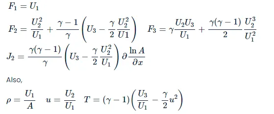
The source term J, the flow vector F, and the solution vector U make up the general version of the governing equations.

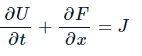
Initial conditions:

When compared to the beginning circumstances and nozzle shape assumed in the non-conservative form of the governing equations outlined above, these alterations are a little more realistic. It is advantageous to start with more improved beginning conditions than those covered before in non-conservative form since it is anticipated that the stability behaviour of the finite-difference formulation utilising the conservation form of the governing equations may be slightly more sensitive.

Assumptions for initial profile of the nozzle :

• For 0≤x′≤0.5">≤x'≤0.5≤x′≤0.5

ρ′">ρ'ρ′ = 1

T' = 1

• For 0.5≤x′≤1.5">≤x'≤1.5≤x′≤1.5

ρ′">ρ'ρ′ = 1.0 - 0.366(x'-0.5)

T' = 1.0 - 0.167(x'-0.5)

• For 0.5≤x′≤1.5">≤x'≤1.5≤x′≤1.5

ρ′">ρ'ρ′ = 0.634 - 0.3879(x'-1.5)

T' = 0.833 - 0.3507(x'-1.5)

Quasi 1-D supersonic flow can be expressed

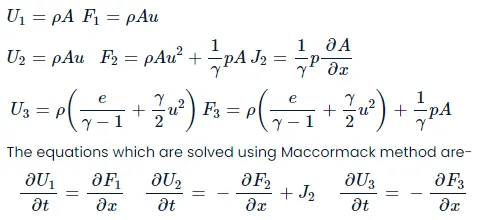
Flux Vector:

Boundary Conditions:

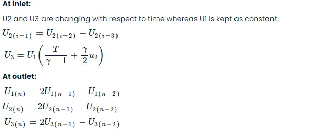
In conservative form, we may allot boundary conditions for inflow and outflow boundary conditions by referring to fig. (b) and absorbing the same way of characteristics approach. The boundary conditions in this instance, nevertheless, will be expressed in terms of solution vectors. Similar to what was previously described, at the subsonic inflow (M1), we need to specify two quantities at the first node, where we have ρ′">ρ'A' and U2= ρ′">ρ'A'V'= 0.59 (Mass flow rate) specified and one quantity will be permitted to float by referring to the left hand characteristic line. It is illogical to establish an outflow boundary condition at the supersonic outflow (M>1) because the information is moving faster than sound. As a result, all dependent variables are left to float and will be computed in time increments.

Matlab Code

clear all
close all
clc

n=31;
nt=1400;
x= linspace(0,3,n);

[rho,Mach,P,t,MassFlow,v,A,rho_th,Mach_th,P_th,t_th,MassFlow_th,v_th] = nonconservation(n,nt);

[rho_c,Mach_c,p_c,T_c,MassFlow_c,v_c,rho_c_th,Mach_c_th,p_c_th,T_c_th,MassFlow_c_th,v_c_th] = conservation(n,nt);



%% NON- CONSERVATION APPROCH AT THROAT
figure(5)
subplot(4,1,1)
plot(P_th)
xlabel("distance")
ylabel("Pressure at throat")
title("Distance vs Pressure")
grid on
hold on
subplot(4,1,2)
plot(t_th)
xlabel("x")
ylabel("temperature at throat")
title("Distance vs temperature")

subplot(4,1,3)
plot(rho_th)
xlabel("distance")
ylabel("density at throat")
title("Distance vs Density")
grid on
hold on

subplot(4,1,4)
plot(Mach_th)
xlabel("distance")
ylabel("Mach number at throat")
title("Distance vs Mach number")
grid on
hold on
% % 

%% CONSERVATIVE APPROACH AT THROAT
figure(6)
subplot(4,1,1)
plot(p_c_th)
xlabel("distance")
ylabel("Pressure at throat")
title("Distance vs Pressure")
grid on
hold on
subplot(4,1,2)
plot(T_c_th)
xlabel("x")
ylabel("temperature at throat")
title("Distance vs temperature")

subplot(4,1,3)
plot(rho_c_th)
xlabel("distance")
ylabel("density at throat")
title("Distance vs Density")
grid on
hold on

subplot(4,1,4)
plot(Mach_c_th)
xlabel("distance")
ylabel("Mach number at throat")
title("Distance vs Mach number")
grid on
hold on





%%%%%%%%%%%%%%%%%%%%%%%%%%%%%%%%%%%%%%%%%%%%%%%%%%%%%%%%%%%%%%%%%%%%%%%%%%%
%%%%%%%%%%%%%%%%%%%%%%%%%%%%%%%%%%%%%%%%%%%%%%%%%%%%%%%%%%%%%%%%%%%%%%%%%%
%%%%%%%%%%%%%        Non Conservative approach            %%%%%%%%%%%%%%%%%
%%%%%%%%%%%%%%%%%%%%%%%%%%%%%%%%%%%%%%%%%%%%%%%%%%%%%%%%%%%%%%%%%%%%%%%%%%%
%%%%%%%%%%%%%%%%%%%%%%%%%%%%%%%%%%%%%%%%%%%%%%%%%%%%%%%%%%%%%%%%%%%%%%%%%%%


function [rho,Mach,P,t,MassFlow,v,A,rho_th,Mach_th,P_th,t_th,MassFlow_th,v_th] = nonconservation(n,nt)


n=31;

x= linspace(0,3,n);
dx = x(2)-x(1);


%input profile

rho = 1-0.3146*x;
t= 1-0.2324*x;
v =  (0.1+1.09*x).*t.^0.5;
A= 1+2.2*(x-1.5).^2;

gamma =1.4;
th =find(A==1);

%time step
nt = 1400;
cfl = 0.5;
dt = min(cfl.*(dx./((sqrt(t))+v)));



for k =1:nt
    rho_old = rho;
    v_old =v;
    t_old =t;


    %predictor step

    for j =2: n-1

        dvdx = (v(j+1)-v(j))/dx;
        drhodx = (rho(j+1)-rho(j))/dx;
        dtdx = (t(j+1)-t(j))/dx;
        dlog_adx = (log(A(j+1)) - log(A(j)))/dx;

        %contiumity equation

        drhodt_p(j) = -rho(j)*dvdx-rho(j)*v(j)*dlog_adx-v(j)*drhodx;

        %momentum euqation

        dvdt_p(j) = -v(j)*dvdx - (1/gamma)*(dtdx +(t(j)/rho(j))*drhodx);

        %energy equation

        dtdt_p(j) = -v(j)*dtdx-(gamma-1)*t(j)*(dvdx+v(j)*dlog_adx);


        %solution update
        rho(j)=rho(j)+drhodt_p(j)*dt;
        v(j) = v(j)+dvdt_p(j)*dt;
        t(j) = t(j)+dtdt_p(j)*dt;

    end

    %corrector step


    for j= 2:n-1

        dvdx = (v(j)-v(j-1))/dx;

        drhodx= (rho(j)-rho(j-1))/dx;

        dtdx = (t(j)-t(j-1))/dx;

        dlog_adx = (log(A(j))-log(A(j-1)))/dx;


        %continuty eqn
        drhodt_c(j) = -rho(j)*dvdx-rho(j)*v(j)*dlog_adx-v(j)*drhodx;

        %momemtum eqn

        dvdt_c(j) = -v(j)*dvdx - (1/gamma)*(dtdx +(t(j)/rho(j))*drhodx);

        %energy eqn

        dtdt_c(j) =-v(j)*dtdx-(gamma-1)*t(j)*(dvdx+v(j)*dlog_adx);


    end

    %aerge of the derivties
    drhodt_avg = 0.5*(drhodt_p+drhodt_c);
    dvdt_avg = 0.5*(dvdt_p+dvdt_c);
    dtdt_avg = 0.5*(dtdt_p+dtdt_c);


    %final solution update

    for  i=2:n-1

        rho(i) = rho_old(i)+drhodt_avg(i)*dt;

        v(i)= v_old(i) +dvdt_avg(i)*dt;

        t(i) = t_old(i)+dtdt_avg(i)*dt;

    end


    %inlet boundary condition
%     rho(1)= 1;
    v(1) = 2*v(2)-v(3);
%     t(1)=1;

    %outlet boundary condition

    v(n)= 2*v(n-1)-v(n-2);
    rho(n) = 2*rho(n-1)-rho(n-2);
    t(n) = 2*t(n-1)-t(n-2);


    MassFlow = rho.*A.*v;
    P= rho.*t;
    Mach = v./t.^0.5;

    %throat values

    rho_th(k) =rho(th);
    v_th(k)= v(th);
    t_th(k) =t(th);
    MassFlow_th(k) =MassFlow(th);
    P_th(k)=P(th);

    Mach_th(k) =Mach(th);









%     resdical values

    v_resv(k) = dvdt_avg(th);
    rho_resv (k)=drhodt_avg(th);
    t_resv(k) =dtdt_avg(th);







        figure(1)
        if k == 50
        plot(x, MassFlow, 'b', 'LineWidth', 1.5)
        hold on
        elseif k == 100
        plot(x, MassFlow, 'r','linewidth', 1.5)
        hold on
        elseif k == 150
        plot(x, MassFlow, 'c', 'LineWidth', 1.5)
        hold on
        elseif k == 200
        plot(x, MassFlow, 'g', 'linewidth', 1.5)
        hold on
        elseif k == 550
        plot(x, MassFlow, 'y', 'linewidth', 1.5)
        hold on
        elseif k == 700
        plot(x, MassFlow, 'k', 'LineWidth', 1.5)
        hold on
        elseif k == 1400
        plot(x, MassFlow,'m', 'LineWidth', 1.5)
        hold on
        grid on
        ylabel('mass flow rate');
        xlabel('nozzle length (x)');
        title('mass flow rate at different time steps Non conservative approach');
        legend('50 time steps','100 time steps','150 time steps','200 time steps', ...
            '550 time steps','700 time steps','1400 time steps');
        end




end
figure (2)
title("nonconservation approch")
subplot(4,1,1)
plot(x,P)
xlabel("distance")
ylabel("Pressure")
title("Distance vs Pressure")
grid on
hold on
subplot(4,1,2)
plot(x,t)
xlabel("x")
ylabel("temperature")
title("Distance vs temperature")

subplot(4,1,3)
plot(x,rho)
xlabel("distance")
ylabel("density")
title("Distance vs Density")
grid on
hold on

subplot(4,1,4)
plot(x,Mach)
xlabel("distance")
ylabel("Mach number")
title("Distance vs Mach number")
grid on
hold on







end






   
%%%%%%%%%%%%%%%%%%%%%%%%%%%%%%%%%%%%%%%%%%%%%%%%%%%%%%%%%%%%%%%%%%%%%%%%%%%
%%%%%%%%%%%%%%%%%%%%%%%%%%%%%%%%%%%%%%%%%%%%%%%%%%%%%%%%%%%%%%%%%%%%%%%%%%
%%%%%%%%%%%%%            Conservative approach            %%%%%%%%%%%%%%%%%
%%%%%%%%%%%%%%%%%%%%%%%%%%%%%%%%%%%%%%%%%%%%%%%%%%%%%%%%%%%%%%%%%%%%%%%%%%%
%%%%%%%%%%%%%%%%%%%%%%%%%%%%%%%%%%%%%%%%%%%%%%%%%%%%%%%%%%%%%%%%%%%%%%%%%%%


function [rho_c,Mach_c,p_c,T_c,MassFlow_c,v_c,rho_c_th,Mach_c_th,p_c_th,T_c_th,MassFlow_c_th,v_c_th] = conservation(n,nt)    



n=31;
L=3;
x=linspace(0,L,n);
dx = x(2)-x(1);

% input profile

A_c= 1+2.2*(x-1.5).^2; %Area



for g=1:n

    if (x(g) >= 0 && x(g) <= 0.5)
    
        rho_c(g) =1.0;
        T_c(g) = 1.0;
    end
    
    if ( x(g) >= 0.5 && x(g) <= 1.5)
    
        rho_c(g) =1.0 -(0.366.*(x(g)-0.5));
        T_c(g)= 1.0 - (0.167.*(x(g)-0.5));
    end
    
    if (x(g)>=1.5 && x(g) <= 3.5)
    
        rho_c(g) = 0.634 - 0.3879*(x(g)-1.5);
        T_c(g)= 0.833 - 0.3507*(x(g)-1.5);
    end
end

v_c =  0.59./(rho_c.*A_c);  %velocity

nt =1400;
gamma =1.4;
%solution variables instalization
u1= rho_c.*A_c;
u2=rho_c.*A_c.*v_c;
u3 =rho_c.*A_c.*(T_c./(gamma-1)+(gamma/2).*v_c.^2);  


for i = 1:nt

    %adative time step dt

    c = 0.5;
    dt = min(c.*dx./(sqrt(T_c)+v_c));

    u1_old =u1;
    u2_old =u2;
    u3_old=u3;


    for j = 2:n-1

        %predictive time step
        f1= u2;
        f2=((u2.^2)./u1) +((gamma-1)/gamma)*(u3-((gamma.*u2.^2)./(2*u1)));
        f3=((gamma.*u2.*u3)./u1)-(gamma*(gamma-1)*(u2.^3)./(2.*u1.^2)); 
     
        J2(j)= (1/gamma)*rho_c(j)*T_c(j).*((A_c(j+1)-A_c(j))/dx);

        %flux function

        df1_dx(j)= (f1(j+1)-f1(j))/dx;
        df2_dx(j)=(f2(j+1)-f2(j))/dx;
        df3_dx(j)=(f3(j+1)-f3(j))/dx;

        %solution function

        du1_dt_p(j)=-df1_dx(j);

        du2_dt_p(j) = -df2_dx(j) +J2(j);

        du3_dt_p(j) = -df3_dx(j);

        %solution update

        u1(j)= u1(j)+du1_dt_p(j)*dt;
        u2(j) =u2(j)+du2_dt_p(j)*dt;
        u3(j) =u3(j)+du3_dt_p(j)*dt;


    end

    for j=2:n-1

        %corretive method
         f1= u2;
        f2=((u2.^2)./u1) +((gamma-1)/gamma)*(u3-((gamma.*u2.^2)./(2*u1))); 
        f3=((gamma.*u2.*u3)./u1)-(gamma*(gamma-1)*(u2.^3)./(2.*u1.^2)); 
       
     
        J2(j)= (1/gamma)*rho_c(j)*T_c(j)*((A_c(j)-A_c(j-1))/dx);

        %flex

        df1_dx(j)= (f1(j)-f1(j-1))/dx;

        df2_dx(j)= (f2(j)-f2(j-1))/dx;

        df3_dx(j) =(f3(j)-f3(j-1))/dx;

        % solution vector

        du1_dt_c(j) = -df1_dx(j); 

        du2_dt_c(j) =-df2_dx(j)+J2(j);  

        du3_dt_c(j) = -df3_dx(j);  

        


    end

    %average of the solution
    du1_dt_avg = 0.5*(du1_dt_p+du1_dt_c);

    du2_dt_avg =0.5*(du2_dt_p+du2_dt_c);

    du3_dt_avg =0.5*(du3_dt_p+du3_dt_c);

    %final solution update

    for k =2:n-1

        u1(k)=u1_old(k)+du1_dt_avg(k)*dt;  % Added old u1,u2,u3 values 

        u2(k) = u2_old(k)+du2_dt_avg(k)*dt;

        u3(k) =u3_old(k)+du3_dt_avg(k)*dt;

    end



    %applying boundary condition
    %inlet boundary condtion

    u1(1)= rho_c(1)*A_c(1);
    u2(1) =(2*u2(2))-u2(3);
    u3(1) =u1(1)*(T_c(1)/(gamma-1)+(gamma/2)*v_c(1)^2); 

    %outlet boundary condition

    u1(n)= 2*u1(n-1)-u1(n-2);

    u2(n)= 2*u2(n-1)-u2(n-2);

    u3(n)= 2*u3(n-1)-u3(n-2);

    %variable update
    rho_c = u1./A_c;  

    v_c =u2./u1;

    T_c= (gamma-1)*((u3./u1) -(gamma/2)*v_c.^2);

    p_c = rho_c.*T_c;

    Mach_c = v_c./T_c.^0.5;

    MassFlow_c = rho_c.*A_c.*v_c;

     %throat values
     th = find(A_c==1);

    rho_c_th(i) =rho_c(th);
    v_c_th(i)= v_c(th);
    T_c_th(i) =T_c(th);
    MassFlow_c_th(i) =MassFlow_c(th);
    p_c_th(i)=p_c(th);

    Mach_c_th(i) =Mach_c(th);


    %graph

     figure(3)
        if i == 50
        plot(x, MassFlow_c, 'b', 'LineWidth', 1.5)
        hold on
        elseif i == 100
        plot(x, MassFlow_c, 'r','linewidth', 1.5)
        hold on
        elseif i == 150
        plot(x, MassFlow_c, 'c', 'LineWidth', 1.5)
        hold on
        elseif i == 200
        plot(x, MassFlow_c, 'g', 'linewidth', 1.5)
        hold on
        elseif i == 550
        plot(x, MassFlow_c, 'y', 'linewidth', 1.5)
        hold on
        elseif i == 700
        plot(x, MassFlow_c, 'k', 'LineWidth', 1.5)
        hold on
        elseif i == 1400
        plot(x, MassFlow_c,'m', 'LineWidth', 1.5)
        hold on
        grid on
        ylabel('mass flow rate');
        xlabel('nozzle length (x)');
        title('mass flow rate at different time steps conservative approach');
        legend('50 time steps','100 time steps','150 time steps','200 time steps','550 time steps','700 time steps','1400 time steps');
        end

end
figure (4)
subplot(4,1,1)
plot(x,p_c)
xlabel("distance")
ylabel("Pressure")
title("Distance vs Pressure")
grid on
hold on
subplot(4,1,2)
plot(x,T_c)
xlabel("x")
ylabel("temperature")
title("Distance vs temperature")

subplot(4,1,3)
plot(x,rho_c)
xlabel("distance")
ylabel("density")
title("Distance vs Density")
grid on
hold on

subplot(4,1,4)
plot(x,Mach_c)
xlabel("distance")
ylabel("Mach number")
title("Distance vs Mach number")
grid on
hold on




end

We entered the number of timesteps and grid points in the function.

The starting condition is computed using these variables.

The predictor and corrector values will then be determined using MacCormack's Technique.

We discover the new remedy.

Use the boundary conditions to determine the following timestep.

The for loop then continues until the given value is reached.

Results:

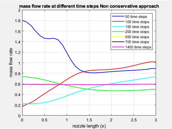
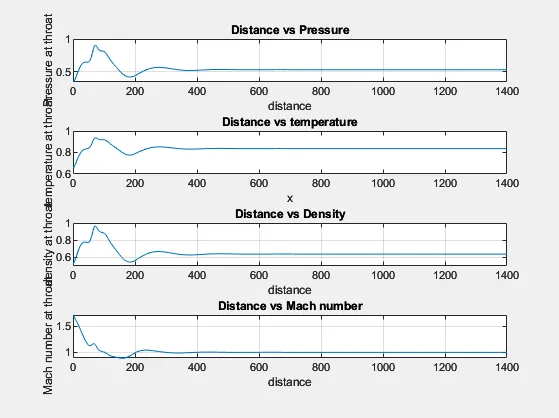
Non- conservative approch:

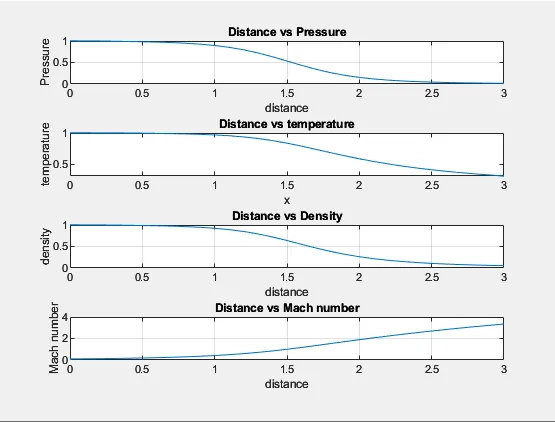
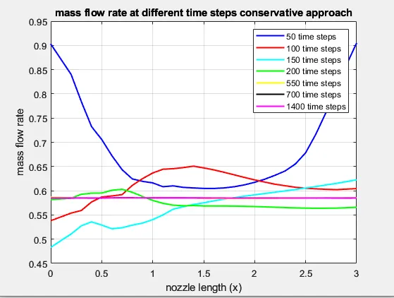
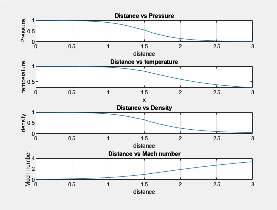
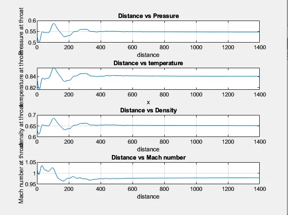
Conservative approach:

	31 grid points (n=16)	31 grid points (n=16)
Flow Variables at Throat	Conservative Form	Non-Conservative Form
Density	0.6517	0.6387
Temperature	0.8407	0.8365
Pressure	0.5479	0.5342
Mach Number	0.9794	0.9994

The aforementioned table includes the analytical, conservative, and non-conservative values for density, temperature, pressure, and mach number at the neck. When we examine the data, we can observe that the non-conservation version's outcomes are far more in line with the real values (That are obtained from the analytical solution). Additionally, we can see that the steady state numerical results are a little bit closer to the exact analytical values than the non-conservation form results, but still not quite there, when the number of grid points is doubled.

Observation:

By examining the graphs of the Distribution of Primitive Variables inside the Nozzle, we can see that the mach number keeps increasing as we move from the intake to the output. At the flow's intake, throat, and outflow, there will be Mach numbers that are less than 1, equal to 1, and greater than 1. The velocity will be lower at the convergent section, but as the pipe cross section increases, the velocity above mach number equal to 1 will rise. The temperature and pressure decrease as the fluid's velocity increases, creating energy as a result. As the pressure rises, so does the density.

A plot of pressure, density, temperature, and mach number at the nozzle throat against the number of time steps shows that the largest changes occur at the earlier times, when the final, steady state value is approaching. Early on, the value of the time derivatives oscillates and is significant. These oscillations are related to a number of unstable compression and expansion waves that move through the nozzle during the transient process. Later, the magnitude of the time derivatives rapidly decreases over a finite number of timesteps.

When comparing the steady state variation of the mass flow obtained using the non-conservation and conservation forms of the governing equation, we can see that the conservation form is substantially more satisfying than that obtained from the non-conservation form. The conservation form results in a distribution that is much closer to being a constant. The non-conservation findings, however, show a wide range, with some deceptive oscillations at the inflow and outflow limits. The conservation form also gets quite near to the accurate analytical solution.

Conclusion:

The distribution of mass flows is improved by using conservation form.
Because they are solved in terms of simple variables and their values are retrieved immediately, non-conservation form is preferable for programming simplicity. However, in conservation form equations, flux variables are used as the units of expression, and the solution vector is solved before the primitive variables, which complicates matters.
Due to the direct computation of basic variables, non-conservative methods are also preferable in terms of accuracy. While in the conservation form, flow variables are used to indirectly calculate primitive variables. More computations will result in more mistakes. When we look at primitive values, this is the situation. However, conservation form is preferable if we are considering flux variables.

In contrast to conservation form, the behaviour of the residuals behaves better in non-conservation form. The residuals deteriorate more quickly in non-conservation form than in conservation form. It is common practise to use the residual decay rate as a gauge of the numerical algorithm's "quality." The non-conservation option is therefore preferred.

The advantage of the non-conservation variant is that the basic variables attain a numerical steady-state faster.

The fact that the dependent variables are not primitive in conservation form but rather in non-conservation form may be the cause. As a result, the simulation time for the non-conservation form is less than that of the conservation form.