Challenge

Week 7 - Simulation of a 1D Super-sonic nozzle flow simulation using Macormack Method

AAatas A G2 Aug 2022

SIMULATION OF A 1D SUPERSONIC NOZZLE FLOW USING MACORMACK METHOD:

The flow at the inlet to the nozzle arrives from the reservoir where the pressure and temperature are denoted by Po and Co. The cross-sectional area of the reservoir is very large and hence the fluid velocity is very low. The flow expands from subsonic to supersonic flow, whereas the velocity of the fluid at the throat is equal to the sonic velocity.

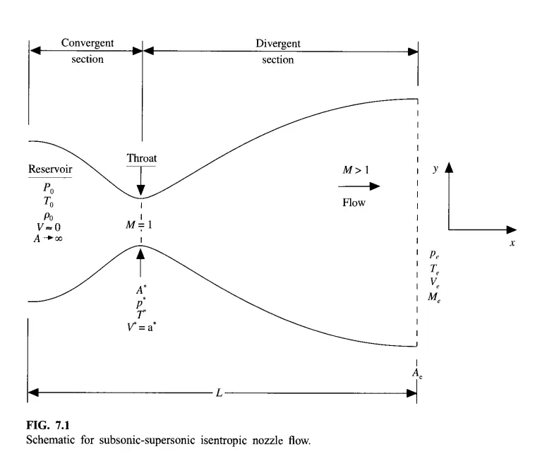
Governing equation

The assumptions made for solving nozzle flow problems is that the flow properties varies only in the x-direction and remains uniform across any given cross-section. This type of problem is called quasi 1D flow problem. The integral form of the governing equations are

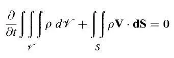
Continuity equation

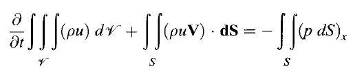
Momentum equation

Energy equations

The integral form of governing equations should be converted into corresponding PDE form such that the PDE can be numerically solved to obtain the primitive variables such as velocity, density, temperature, pressure and so on. A control volume of negligible dimensions (tending to zero) is selected and the above integral form of governing equation is applied to CV and solved to obtain both conservative and non-conservative form of PDE.

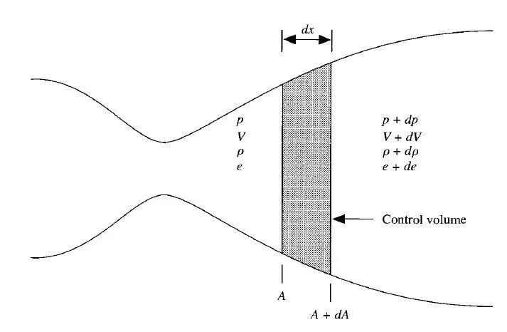
Conservative form of governing equation

Continuity equation

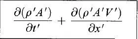
Momentum equation

Energy equation

Non-Conservative form of Governing equation

Continuity equation

Momentum equation

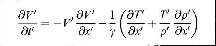
Energy equation

, , , , ,,

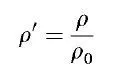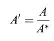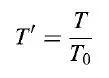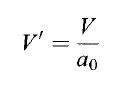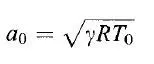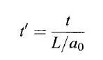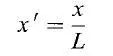
The prime in the above equations represents the non-dimensional form of governing equation. Non-dimensional form of Navier stokes equation can ease the analysis of the problem and it reduces the number of parameters.

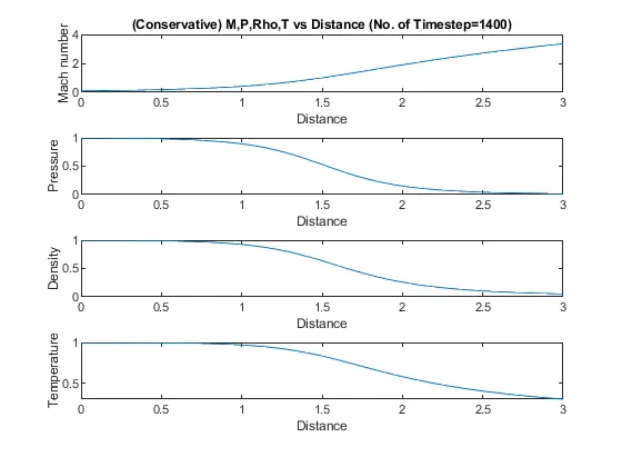
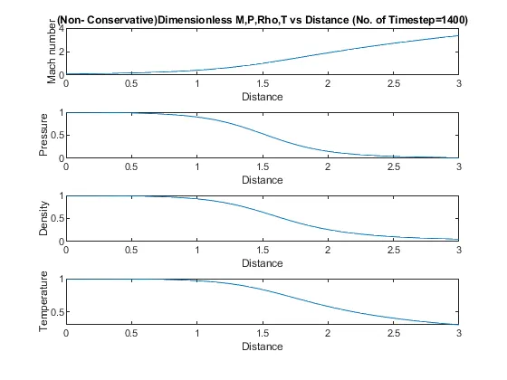
The difference between the conservative and non-conservative form of governing equation is that both forms give the same analytical solution but the different numerical output. Conservative form provides accurate results and it can provide better results in the presence of shocks or discontinuities.

Steps for solving the Nozzle flow problem

Meshing

The given 1D domain is divided into n number of elements. For Nozzle flow problem the length of nozzle is chosen as 3 and the length is divided into 30 elements.

Discretization

The PDE is discretized and solved for the points in the domain. Maccormack method is used for discretizing the equation. Maccormack method gives better results for the hyperbolic equation and it is also called as a shock-capturing method. These methods can provide stable solutions in the presence of shock. Hence they are used in nozzle flow problems. In Maccormack method combination of both forward and backward differencing schemes can be used to solve for the primitive variables. Non-conservative and conservative form of governing equations are solved by using this method.

The time step used for the simulation is

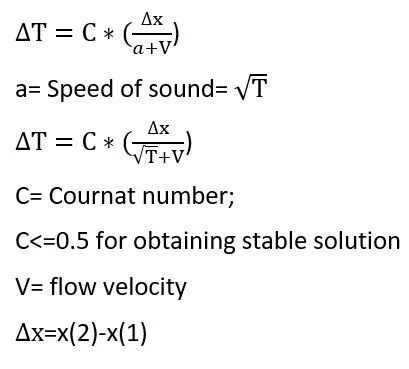
The minimum value of is used such that the time marching solution is following the actual unsteady flow variation that exists in nature.

Steps involved in Macormack method

Predictor step(forward differencing)
Solution update
Corrector step( Backward differencing)
Determining the average of the time derivative
Final solution update

Non-conservative form of Governing equation

In the non-conservative form of governing equation the continuity, momentum and energy equations can be discretized directly to obtain the primitive variables such as density, velocity and temperature.

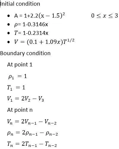
The initial and boundary conditions are

Conservative form of governing equation

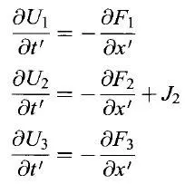
In the conservative form of governing equation, the primitive variables are grouped and they are represented in terms of solution vector U, flux vector F and source term J. The resulting equation is solved to obtain updated values of the density, velocity, temperature and so on.

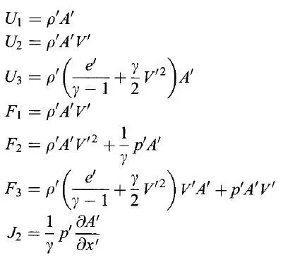
Now the governing equation can be written as

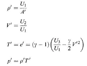
To obtain the primitive variables the solution vector U1, U2, U3 must be decoded.

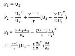
It is better to write F1, F2, F3 in terms of U1, U2, U3 to avoid the occurrence of instabilities during the time marching solution.

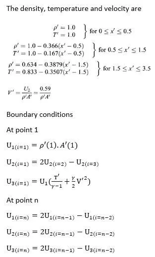
The initial and boundary condition for the conservative form of governing equations are

Initial conditions

MATLAB CODE:

1) Main code 

 

clear all
close all
clc

n=input('Enter number of grid points ');
x=linspace(0,3,n);
gamma=1.4;
dx=x(2)-x(1);





%area
 a=1+(2.2*(x-1.5).^2);

% timestep
nt=1400;


% Non -conservative 
[rho,v,t,M,p,m,p_t,rho_t,t_t,M_t]=non_conservative(n,nt);

%Conservative
[rho_c,v_c,t_c,M_c,p_c,m_c,p_tc,rho_tc,t_tc,M_tc]= conservative(n,nt);


% Non -conservative

% To plot variables Vs distance
figure(1)
subplot (4,1,1)
plot(x,M)
title_text=sprintf('(Non- Conservative)Dimensionless M,P,Rho,T vs Distance (No. of Timestep=%d)',nt);
title(title_text)
xlabel('Distance')
ylabel('Mach number')
hold on

subplot(4,1,2)
plot(x,p)
xlabel('Distance')
ylabel('Pressure')
hold on
   
subplot(4,1,3)
plot(x,rho)
xlabel('Distance')
ylabel('Density')
 hold on  

subplot(4,1,4)
plot(x,t)
xlabel('Distance')
ylabel('Temperature')
hold on 

% To plot variables at time step 
figure(2)
nt=1:1400 ;
subplot(4,1,1)
plot (nt,t_t)
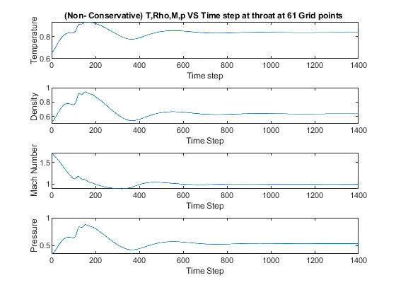
 title_text=sprintf( '(Non- Conservative) T,Rho,M,p VS Time step at throat at %d Grid points ',n)
 title(title_text)
xlabel('Time step')
ylabel('Temperature')
hold on


subplot(4,1,2)
plot(nt,rho_t)
xlabel('Time Step')
ylabel('Density ')
hold on

subplot(4,1,3)
plot(nt,M_t)
xlabel('Time Step')
ylabel('Mach Number')
hold on

subplot(4,1,4)
plot(nt,p_t)
xlabel('Time Step')
ylabel('Pressure')
hold on


% Conservative 
nt=1400 ;
figure(3)
subplot(4,1,1)
plot(x,M_c)
title_text=sprintf('(Conservative) M,P,Rho,T vs Distance (No. of Timestep=%d)',nt)
title(title_text)
xlabel('Distance')
ylabel('Mach number')
hold on

subplot(4,1,2)   
plot(x,p_c)

xlabel('Distance')
ylabel('Pressure')
hold on
   
subplot(4,1,3)
plot(x,rho_c)
xlabel('Distance')
ylabel('Density')
hold on
   
subplot(4,1,4)
plot(x,t_c)

xlabel('Distance')
ylabel('Temperature')
hold on

figure(4)
nt=1:1400 ;
subplot(4,1,1)
plot (nt,t_tc)
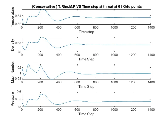
title_text=sprintf( ' (Conservative ) T,Rho,M,P VS Time step at throat at %d Grid points',n)
title(title_text)
xlabel('Time step')
ylabel('Temperature')
hold on

subplot(4,1,2)
plot(nt,rho_tc)

xlabel('Time Step')
ylabel('Density ')
hold on

subplot(4,1,3)
plot(nt,M_tc)

xlabel('Time Step')
ylabel('Mach Number')
hold on

subplot(4,1,4)
plot(nt,p_tc)

xlabel('Time Step');
ylabel('Pressure');
hold on

figure(7)
plot(x,m_c)
hold on
plot(x,m)
line([0 3],[0.579 0.579],'linewidth',2,'color','g');
title_text=sprintf( 'Mass flow rate Vs Distance for  %d Grid points',n);
title(title_text);
legend ('Conservative','Non-Conservative', 'Analytical Solution');
xlabel('x/L');
ylabel('Mass flow rate m');


 2) Code  for conservative form

function[rho_c,v_c,t_c,M_c,p_c,m_c,p_tc,rho_tc,t_tc,M_tc]= conservative(n,nt)

x=linspace(0,3,n);
gamma=1.4;
dx=x(2)-x(1);





%area
 a=1+(2.2*(x-1.5).^2);

%area
 a=1+(2.2*(x-1.5).^2);




    
for i=1:length(x)
       
if (x(i)>=0)&&(x(i)<=0.5)
    rho(i)=1;
    t(i)=1;

elseif (x(i)>=.5)&&(x(i)<=1.5)
        
        rho(i)=1-.366.*(x(i)-0.5);
        t(i)=1-.167.*(x(i)-0.5);
else
     rho(i)=.634-.3879.*(x(i)-1.5) ;
     t(i)=.833-.3507.*(x(i)-1.5);
 end
end


 



a=1+(2.2*(x-1.5).^2);
  v=(0.59)./(rho.*a);
  
  
   
    U1=rho.*a; 

    U2=rho.*a.*v ; 
    U3= rho.*((t./(gamma-1)) + ((gamma/2).*v.^2)).*a;
    
    
    
     
  delta_t= 0.5*(dx./(sqrt(t)+v));
 
  dt=min(delta_t);
  
  

for k=1:nt
   
  U1_old=U1;
  U2_old=U2;
  U3_old=U3;
  
 
    


    F1=U2;
    F2=((U2.^2)./U1)+((gamma-1)/gamma)*(U3-(gamma/2)*((U2.^2)./U1));
    F3=(gamma*(U2.*U3)./U1)-((gamma*(gamma-1))/2)*((U2.^3)./(U1.^2));



  
%% Predictor
for j=2:n-1
  
  J(j)=(1/gamma)*rho(j)*t(j)*((a(j+1)-a(j))/dx);



 
 dU1dt_p(j)= -((F1(j+1)-F1(j))/dx);
 dU2dt_p(j)=-((F2(j+1)-F2(j))/dx)+J(j) ;
 dU3dt_p(j)= -((F3(j+1)-F3(j))/dx);
 
 
 U1(j)=U1_old(j)+(dU1dt_p(j))*dt;
 U2(j)=U2_old(j)+(dU2dt_p(j))*dt;
 U3(j)=U3_old(j)+(dU3dt_p(j))*dt;

end




rho=U1./a ;
v= U2./U1;
t=(gamma-1)*((U3./U1)-((gamma/2)*(v.^2)));
 


% for i=1:length(n)
%       delta_t(i)= 0.5*(dx(i)/sqrt(t(i))*v(i));
%   end
%   dt=min(delta_t);
  

%Update

%     
% F1=U2;
% F2=U2.^2./U1+((gamma-1)/gamma)*(U3-(gamma/2).*(U2.^2./U1));
% F3=((gamma*U3.*U2)/U1)-((gamma*(gamma-1)/2)*(U2.^3./U1.^2));

    F1=U2;
    F2=((U2.^2)./U1)+((gamma-1)/gamma)*(U3-(gamma/2)*(((U2).^2)./U1));
    F3=(((gamma)*(U2.*U3))./U1)-(((gamma*(gamma-1))/2)*((U2.^3)./U1.^2));



  % corrector  
 for q=2:n-1
   
   J(q)=(1/gamma)*rho(q)*t(q)*((a(q)-a(q-1))/dx)
  
   
  dU1dt_c(q)= -(F1(q)-F1(q-1))/dx;
  dU2dt_c(q)=-((F2(q)-F2(q-1))/dx)+J(q) ;
  dU3dt_c(q)= -(F3(q)-F3(q-1))/dx;
 end
 
 
  dU1dt_av= 0.5*(dU1dt_p+dU1dt_c);
  dU2dt_av=0.5*(dU2dt_p+dU2dt_c);
  dU3dt_av=0.5*(dU3dt_p+dU3dt_c);
  
 
  
  for m=2:n-1
      
  U1(m)=U1_old(m)+(dU1dt_av(m)*dt);
  U2(m)=U2_old(m)+(dU2dt_av(m)*dt);
  U3(m)=U3_old(m)+(dU3dt_av(m)*dt);
  end
  
  
        %Defining Inletflow Boundary conditions
        U1(1)=rho(1)*a(1);
        U2(1) = 2*U2(2)-U2(3);
        v(1)=U2(1)/U1(1);
        U3(1) = U1(1)*(t(1)/(gamma-1)+(gamma/2)*v(1)^2);


        %Defining outflow Boundary conditions

        U1(n)=2*U1(n-1)-U1(n-2);

        U2(n)=2*U2(n-1)-U2(n-2);

        U3(n)=2*U3(n-1)-U3(n-2);
       
      rho=U1./a;
      v=(U2./U1);
      t=(gamma-1)*((U3./U1)-(gamma/2)*(U2./U1).^2);
     
       
    %Mach Number
    M=(v./sqrt(t));
   
    %Pressure
    p=rho.*t;
    
    % Mass flow rate
    m=rho.*v.*a;

  
  throat=find(a==1);
  p_t(k)=p(throat);
  rho_t(k)=rho(throat) ; 
  t_t(k)=t(throat);
  M_t(k)=M(throat);
 % m_t(k)=m(throat);
 
 figure(6)
       hold on
           if k==50
                plot(x,m,'b')
           elseif k==100
                plot(x,m,'g')
           elseif k==150
                plot(x,m,'y')
           elseif k==200
                plot(x,m,'m')
           elseif k==700
                plot(x,m,'c')
                title('(Conservative)Mass flow rate Vs Distance')
                legend('50','100','150','200','700')
                xlabel('Non-dimensional distance through nozzle (x)')
                ylabel('Mass flow rate (rho.A.V)')
           end

end
rho_c=rho;
v_c=v;
t_c=t;
M_c=M;
p_c=p;
m_c=m;
p_tc=p_t;
rho_tc=rho_t;
t_tc=t_t;
M_tc=M_t;
%m_tc=m_t;

end
3) Code for non-conservative form

function[rho,v,t,M,p,m,p_t,rho_t,t_t,M_t]= non_conservative(n,nt)
x=linspace(0,3,n);
gamma=1.4;
dx=x(2)-x(1);

%area
 a=1+(2.2*(x-1.5).^2);

%calculate initial profile
rho=1-0.3146*x;
%temperature
t=1-0.2314*x;
v=(.1+1.09*x).*t.^0.5;

%area
a=1+2.2*(x-1.5).^2;

%timesteps
nt=1400;
dt=0.02;

   
  delta_t= 0.5*(dx./(sqrt(t)+v));
 
  dt=min(delta_t);

% % Outer time loop
for k=1:nt 
    % Predictor
    rho_old=rho;
    v_old=v;
    t_old=t;
    
for j=2:n-1
    
%drho_dt_p=
dvdx=(v(j+1)-v(j))/dx;
drhodx=(rho(j+1)-rho(j))/dx;
dtdx=(t(j+1)-t(j))/dx;
dlogadx=(log(a(j+1))-log(a(j)))/dx;
%Continuity equation
drhodt_p(j)=-rho(j)*dvdx -rho(j)*v(j)*dlogadx-v(j)*drhodx;

%Momentum Equation
dvdt_p(j)= -v(j)*dvdx - ((1/gamma)*(dtdx + (t(j)/rho(j)*drhodx)));

%Energy Equation
dTdt_p(j)= -v(j)*dtdx-(gamma-1)*t(j)*(dvdx+v(j)*dlogadx);

%Solution Update
v(j)=v(j)+dvdt_p(j)*dt;
rho(j)=rho(j)+drhodt_p(j)*dt;
t(j)=t(j)+dTdt_p(j)*dt;
end
  
    
    
    % Corrector Method
for j=2:n-1
    
%drho_dt_p=
dvdx=(v(j)-v(j-1))/dx;
drhodx=(rho(j)-rho(j-1))/dx;
dtdx=(t(j)-t(j-1))/dx;
dlogadx=(log(a(j))-log(a(j-1)))/dx;
%Continuity equation
drhodt_c(j)=-rho(j)*dvdx -rho(j)*v(j)*dlogadx-v(j)*drhodx;

%Momentum Equation
dvdt_c(j)= -v(j)*dvdx - ((1/gamma)*(dtdx + (t(j)/rho(j)*drhodx)));

%Energy Equation
dTdt_c(j)= -v(j)*dtdx-(gamma-1)*t(j)*(dvdx+v(j)*dlogadx);

% %Solution Update
% v(j)=v(j)+dvdt_p(j)*dt;
% rho(j)=rho(j)+drhodt_p(j)*dt;
% t(j)=t(j)+dTdt_p(j)*dt;
end
  
% Compute the average

drhodt_a= 0.5 *(drhodt_p+drhodt_c)
dvdt_a= 0.5*(dvdt_p+dvdt_c)
dTdt_a=0.5*(dTdt_p+dTdt_c)

for i=2:n-1
   % Final solution update 
 v(i)=v_old(i)+dvdt_a(i)*dt;
 rho(i)=rho_old(i)+drhodt_a(i)*dt;
 t(i)=t_old(i)+dTdt_a(i)*dt;
end

% Apply Boundary COndition
% Inlet
v(1)=2*v(2)-v(3);

%outlet
v(n)=2*v(n-1)-v(n-2);
t(n)=2*t(n-1)-t(n-2);
rho(n)=2*rho(n-1)-rho(n-2);


% mach number

M=(v./sqrt(t));

% Density
p=rho.*t ;

% Mass flow
m=rho.*v.*a;

  
  throat=find(a==1);
  p_t(k)=p(throat);
  rho_t(k)=rho(throat) ; 
  t_t(k)=t(throat);
  M_t(k)=M(throat);
%  m_t(k)=M(throat);

figure(5)
       hold on
           if k==50
                plot(x,m,'b')
           elseif k==100
                plot(x,m,'g')
           elseif k==150
                plot(x,m,'y')
           elseif k==200
                plot(x,m,'m')
           elseif k==700
                plot(x,m,'c')
                title('(Non-Conservative) Mass flow rate Vs Distance')
                legend('50','100','150','200','700')
                xlabel('Non-dimensional distance through nozzle (x)')
                ylabel('Mass flow rate (rho.A.V)')
           end
end

end

RESULTS AND DISCUSSION:

1) Steady-state distribution of primitive variables inside the nozzle

2)Time wice variation of primitive variable

3) Variation of Mass flow rate distribution inside the nozzle at different time steps during the time-marching process

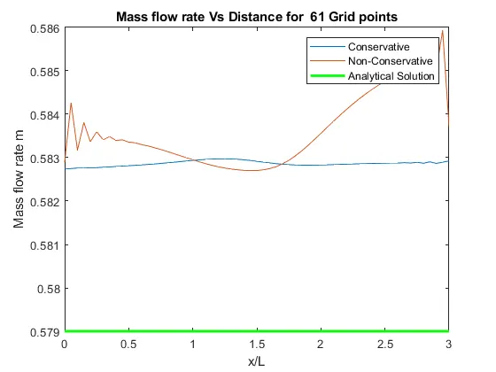
4) Comparison of Normalized mass flow rate distributions of both forms

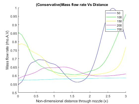
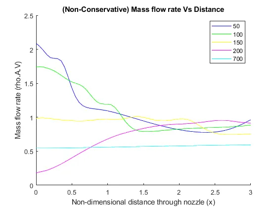
5) Grid independence test

Sl No	n=31	n=61
Conservative	@throat :n=16	@throat: n=31
Pressure	0.5487	0.5340
Velocity	0.8969	0.9121
Temperature	0.8410	0.8355
Density	0.6524	0.6391
Mach number	0.9780	0.9979
Non-Conservative
Pressure	0.5342	0.5327
Velocity	0.9140	0.9138
Temperature	0.8365	0.8345
Density	0.6378	0.6377
Mach Number	0.9994	0.9998

Conclusion:

The non-conservative form produces accurate results for the primitive variable and the conservative form gives better results for the flux variable.

Week 7 - Simulation of a 1D Super-sonic nozzle flow simulation using Macormack Method

Ship work like this
in your own course.

Talk to a career counsellor

Ship work like thisin your own course.

Talk to a career counsellor

Ship work like this
in your own course.