Week 7 - Simulation of a 1D Super-sonic nozzle flow simulation using Macormack Method
The objective of this problem is to simulate the isentropic flow through a quasi 1D subsonic supersonic nozzle using conservative and non conservative form of governing equations:
We have considered the the study of isentropic flow through a convergent divergent nozzle.The cross section area of the opening is very large copared to the throat of the nozzle ,hence the velocity is very small. The flow is locally subsonic to the convergent section of the nozzle, sonic at the throat and supersonic at the divergent section.
We assume that at a given section area ia A, the flow properties are uniform across the section, hence although the area of the nozzle changes as distance changes, we make assumption that the flow properties varies along x direction only because at any particular cross section properties of flow is constant. Such flows are defined as quasi 1D flow.
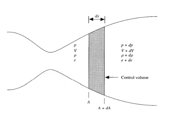
Here is the figure:
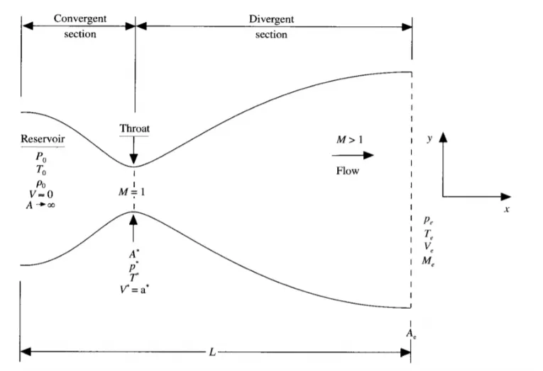
A differential length and elemental variation of parameters.
These equations are solved by Macormack method using time marching process.
Macormack method:
Let f(x) is the equation we are required to solve. Then the following steps are to be followed.
1)Initial profile:
BEfore performing the calculation, the initial flow variables (velocity, density, temperature) has to be known. We start these values as guess values with carefulness.
Predictor step:
Solution update: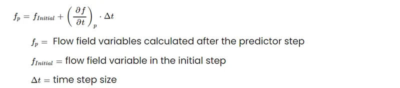
Corrector step: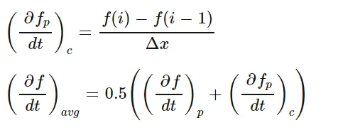
Final solution update:
f_sol = Final solution of the flow field variables for the 1st time step.
Matlab code:
close all;
clear all;
clc
L = 3;%%length of nozzle
n = [31 62 93];
nt = 1:1400;
cfl = 0.5;
for i = 1:length(n)
x = linspace(0,L,n(i));
[mfr_nc,mfr_throat_nc] = non_conservative(L,n(i),nt,cfl);
[mfr_c,mfr_throat_c] = conservative(L,n(i),nt,cfl);
figure(7)
subplot(2,1,1)
plot(nt,mfr_throat_c,'b',nt,mfr_throat_nc,'r','lineWidth',2)
xlabel('Time steps(nt)')
ylabel('Mass flow rate')
legend('Consevative form','Non-conservative form')
title('Mass flow rate using "Non conservative v/s Conservative form" at throat point i=16')
subplot(2,1,2)
plot(x,mfr_c,'b',x,mfr_nc,'r','linewidth',2)
xlabel('Length of nozzle')
ylabel('Mass flow rate')
legend('Consevative form','Non-conservative form')
title('Mass flow rate using "Non conservative v/s Conservative form" in the nozzle')
figure(8)
subplot(2,1,1)
plot(nt,mfr_throat_c,'linewidth',2)
xlabel('Time steps(nt)')
ylabel('Mass flow rate')
legend('@31 nodes','@62 nodes','@93 nodes')
title('Conservatiev from:Grid independency test at throat point i=16')
subplot(2,1,2)
plot(nt,mfr_throat_nc,'linewidth',2)
hold on
xlabel('Time steps(nt)')
ylabel('Mass flow rate')
legend('@31 nodes','@62 nodes','@93 nodes')
title('Non-conservatiev from:Grid independency test at throat point i=16')
figure(9)
subplot(2,1,1)
plot(x,mfr_c,'linewidth',2)
hold on
xlabel('Length of nozzle')
ylabel('Mass flow rate')
legend('@31 nodes','@62 nodes','@93 nodes')
title('Conservatiev from:Grid independency test along the nozzle')
subplot(2,1,2)
plot(x,mfr_nc,'linewidth',2)
hold on
xlabel('Length of nozzle')
ylabel('Mass flow rate')
legend('@31 nodes','@62 nodes','@93 nodes')
title('Non_conservatiev from:Grid independency test at along the nozzle')
end
Non-consevative form:
function[mfr_nc,mfr_throat_nc]=non_conservative(L,n,nt,cfl)
x = linspace(0,L,n);
dx = x(2)-x(1);
%%initial conditions rho ,a,v,T,mfr ,M,p
rho = 1-0.3146*x;
T = 1-0.2314*x;
v = (0.1+1.09*x).*T.^0.5;
a = 1+2.2*(x-1.5).^2;
M = v./(T.^0.5);
mfr = rho.*a.*v;
p = rho.*T;
gamma = 1.4;
for z=1:31
u=(T(z))^(1/2);
dt(z) = cfl*dx/(u+v(z));
end
dt = min(dt);
for i=1:length(nt)
%storing initial values
rho_old = rho;
T_old = T;
v_old = v;
for j = 2:n-1
%predictor step
d_rho_dx = (rho(j+1)-rho(j))/dx;
d_v_dx = (v(j+1)-v(j))/dx;
d_T_dx = (T(j+1)-T(j))/dx;
d_a_dx = (log(a(j+1))-log(a(j)))/dx;
d_rho_dt_p(j) = -rho(j)*d_v_dx-rho(j)*v(j)*d_a_dx-v(j)*d_rho_dx;%continuity
d_v_dt_p(j) = -v(j)*d_v_dx-(1/gamma)*(d_T_dx+(T(j)/rho(j))*d_rho_dx);%momentum
d_T_dt_p(j) = -v(j)*d_T_dx-(gamma-1)*T(j)*(d_v_dx+v(j)*d_a_dx);%energy
%%updating primitives
v(j) = v_old(j)+d_v_dt_p(j)*dt;
rho(j) = rho_old(j)+d_rho_dt_p(j)*dt;
T(j) = T_old(j)+d_T_dt_p(j)*dt;
%%corrector step
d_rho_dx = (rho(j)-rho(j-1))/dx;
d_v_dx = (v(j)-v(j-1))/dx;
d_T_dx = (T(j)-T(j-1))/dx;
d_a_dx = (log(a(j))-log(a(j-1)))/dx;
d_rho_dt_c(j) = -rho(j)*d_v_dx-rho(j)*v(j)*d_a_dx-v(j)*d_rho_dx;%continuity
d_v_dt_c(j) = -v(j)*d_v_dx-(1/gamma)*(d_T_dx+(T(j)/rho(j))*d_rho_dx);%momentum
d_T_dt_c(j) = -v(j)*d_T_dx-(gamma-1)*T(j)*(d_v_dx+v(j)*d_a_dx);%energy
end
%%average time derivatives
d_rho_dt_avg = 0.5*(d_rho_dt_p+d_rho_dt_c);
d_v_dt_avg = 0.5*(d_v_dt_p+d_v_dt_c);
d_T_dt_avg = 0.5*(d_T_dt_p+d_T_dt_c);
%final corrected vallues
for k = 2:n-1
rho(k) = rho_old(k)+d_rho_dt_avg(k)*dt;
v(k) = v_old(k)+d_v_dt_avg(k)*dt;
T(k) = T_old(k)+d_T_dt_avg(k)*dt;
end
%%boundary condition at entry
v(1)=2*v(2)-v(3);
%%boundary condition at exit
v(n) = 2*v(n-1)-v(n-2);
rho(n) = 2*rho(n-1)-rho(n-2);
T(n) = 2*T(n-1)-T(n-2);
%final update of primitives
p = rho.*T;
M = v./T.^0.5;
error(k) = abs(v(k)-v(k-1));
mfr = rho.*a.*v;
%to find values at throat point
T_throat(i) = T(16);
rho_throat(i) = rho(16);
v_throat(i) = v(16);
M_throat(i) = M(16);
error_throat(i) = error(16);
mfr_throat(i) = mfr(16);
p_throat(i)=p(16);
if n==31
for ii=[1:50:201 700]
if ii==i
figure(1)
plot(x,mfr,'linewidth',2)
hold on
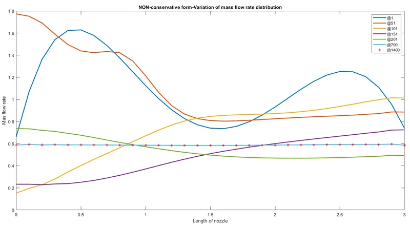
title('NON-conservative form-Variation of mass flow rate distribution')
xlabel('Length of nozzle')
ylabel('Mas flow rate')
elseif i==1400
plot(x,mfr,'*r')
legend('@1','@51','@101','@151','@201','@700','@1400')
end
end
end
end
if n==31
figure(2)
plot(x,v,'b',x,p,'r',x,T,'k',x,rho,'m',x,M,'g',x,mfr,'c')
ylim([-0.1 3.7])
title(sprintf('Time step = %d',i))
xlabel('Length of nozzle')
ylabel('Non dimensional parameters')
legend('Velocity','Pressure','Temperature','Density','MAch Number','Mass flow rate','location','northwest')
title('Non -conservative form-Steady state distrinution of primitive variables inside the nozzle')
figure(3)
plot(nt,rho_throat)
hold on
plot(nt,v_throat,'linewidth',2)
plot(nt,p_throat,'linewidth',2)
plot(nt,T_throat,'linewidth',2)
plot(nt,M_throat,'linewidth',2)
plot(nt,mfr_throat,'linewidth',2)
xlabel('Time steps(nt)')
ylabel('Non-dimensional parameters')
legend('Density','Velocity','Pressure','Temperature','Mach number','Mass flow rate')
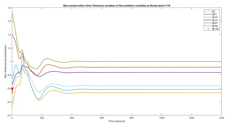
title('Non-conservative form-Timewise variation of the primitive variables at throat point i=16')
end
mfr_nc = mfr;
mfr_throat_nc = mfr_throat;
end
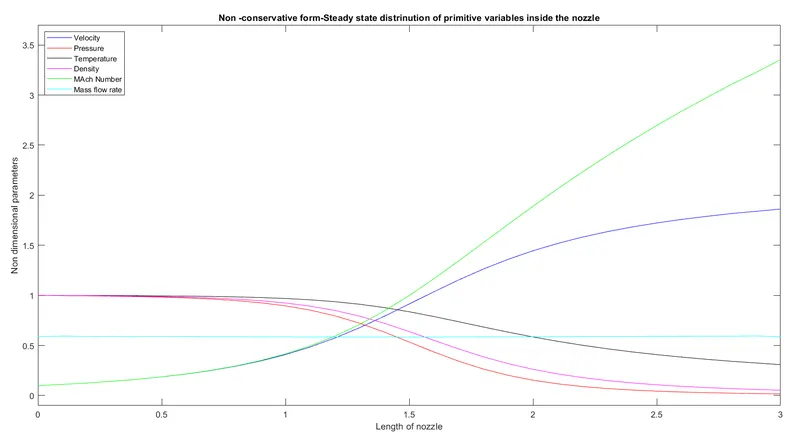
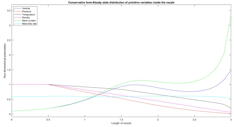
This figure shows the variation of flow parameters along the length of nozzle.
Mach number and velocity increases while the other parameters decreases.
Conservative form:
function[mfr_c,mfr_throat_c]=conservative(L,n,nt,cfl)
x=linspace(0,L,n);
dx = x(2)-x(1);
%initial conditions rho, a, v, T, mfr, p
for ii=1:length(x)
if(x(ii)<=0.5)
rho(ii)=1;
T(ii) = 1;
elseif (x(ii)>0.5) & (x(ii)<=1.5)
rho(ii)=1-0.366*(x(ii)-0.5);
T(ii)=1-0.167*(x(ii)-0.5);
elseif (x(ii)>1.5) & (x(ii)<=3.5)
rho(ii) = 0.634-0.3879*(x(ii)-1.5);
T(ii) = 0.833-0.3507*(x(ii)-1.5);
end
end
a = 1+2.2*(x-1.5).^2;
gamma = 1.4;
%solution vectors
u1 = rho.*a;
u2 = 0.59*ones(1,n);
v = u2./u1;
u3 = u1.*((T./(gamma-1))+(gamma/2).*v.^2);
M = v./(T.^0.5);
mfr = rho.*a.*v;
p = rho.*T;
for z=1:31
u=(T(z))^(1/2);
dt(z) = cfl*dx/(u+v(z));
end
dt = min(dt);
for i=length(nt)
%storing initial values
u1_old = u1;
u2_old = u2;
u3_old = u3;
for j=2:n-1
%flux vectors
f1 = u2;
f2 = ((u2.^2)./u1)+((gamma-1)/gamma)*(u3-((gamma/2)*(u2.^2)./u1));
f3 = ((gamma.*u2.*u3)./u1)-((gamma*(gamma-1)/2)*(u2.^3)./(u1.^2));
%%source term
j1 = (1/gamma)*rho(j)*T(j)*((a(j+1)-a(j))/dx);
%predictor term
d_u1_dt_p(j) = -(f1(j+1)-f1(j))/dx;
d_u2_dt_p(j) = -(f2(j+1)-f2(j))/dx+j1;
d_u3_dt_p(j) = -(f3(j+1)-f3(j))/dx;
%%updating solution vectors
u1(j) = u1_old(j) + d_u1_dt_p(j)*dt;
u2(j) = u2_old(j) + d_u2_dt_p(j)*dt;
u3(j) = u3_old(j) + d_u3_dt_p(j)*dt;
%%updating primitives
rho = u1./a;
T = (gamma-1).*(u3./u1-(gamma/2).*(u2./u1).^2);
%updating flux terms
f1 = u2;
f2 = u2.^2./u1+((gamma-1)/gamma).*(u3-(gamma/2)*u2.^2./u1);
f3 = gamma.*u2.*u3./u1-0.5*gamma*(gamma-1).*u2.^3./u1.^2;
%source term for corrector step
j2 = (1/gamma)*(rho(j)*T(j)*(a(j)-a(j-1))/dx);
%corrector step
d_u1_dt_c(j) = -(f1(j)-f1(j-1))/dx;
d_u2_dt_c(j) = -(f2(j)-f2(j-1))/dx+j2;
d_u3_dt_c(j) = -(f3(j)-f3(j-1))/dx;
end
%average time derivatives
d_u1_dt_avg = 0.5*(d_u1_dt_p + d_u1_dt_c);
d_u2_dt_avg = 0.5*(d_u2_dt_p + d_u2_dt_c);
d_u3_dt_avg = 0.5*(d_u3_dt_p + d_u3_dt_c);
%%final corrected values
for k=2:n-1
u1(k) = u1_old(k) + d_u1_dt_avg(k)*dt;
u2(k) = u2_old(k) + d_u2_dt_avg(k)*dt;
u3(k) = u3_old(k) + d_u3_dt_avg(k)*dt;
end
%%entry boundary conditions
u1(1) = a(1);
u2(1) = 2*u2(2)-u2(3);
u3(1) = u1(1)*(T(1)/(gamma-1) + (gamma*(u2(1)/u1(1))^2)/2);
%%exit boundary condition
u1(n) = 2*u1(n-1)-u1(n-2);
u2(n) = 2*u2(n-1)-u2(n-2);
u3(n) = 2*u3(n-1)-u3(n-2);
%%final update of primitives
rho = u1./a;
v = u2./u1;
T = (gamma-1).*(u3./u1-(gamma/2).*(u2./u1).^2);
p = rho.*T;
M = v./T.^0.5;
error(k) = abs(v(k)-v(k-1));
mfr = u2;
%%to find values at throat point
T_throat(i)=T(16);
rho_throat(i)=rho(16);
v_throat(i)=v(16);
M_throat(i)=M(16);
p_throat(i)=p(16);
error_throat(i)=error(16);
mfr_throat(i)=mfr(16);
if n==31
for ii=[1:50:201 700]
if ii==i
figure(4)
plot(x,mfr,'linewidth',2)
hold on
title('Conservative form-Variation of mfr inside the nozzle')
xlabel('Length of nozzle')
ylabel('Mass flow rate')
elseif i==1400
plot(x,mfr,'*r')
legend('@1','@51','@101','@151','@201','@700','@1400')
end
end
end
end
if n==31
figure(5)
plot(x,v,'b',x,p,'r',x,T,'k',x,rho,'m',x,M,'g',x,mfr,'c')
ylim([-0.1 3.7])
title(sprintf('Timestep = %d',i))
xlabel('Length of nozzle')
ylabel('Non dimensional parameters')
legend('Velocity','Pressure','Temperature','Density','Mach number','Mass flow rate','location','northwest')
title('Conservative form-Steady state distribution of primitive variables inside the nozzle')
figure(6)
plot(nt,rho_throat)
hold on
plot(nt,v_throat,'linewidth',2)
hold on
plot(nt,p_throat,'linewidth',2)
hold on
plot(nt,T_throat,'linewidth',2)
hold on
plot(nt,M_throat,'linewidth',2)
hold on
plot(nt,mfr_throat,'linewidth',2)
xlabel('Time steps (nt)')
ylabel('Non dimensional parameters')
legend('Density','Velocity','Pressure','Temperature','Mach number','Mass flow rate')
title('Conservative form-Timewise variation')
end
mfr_c = mfr;
mfr_throat_c = mfr_throat;
end