Week 7 - Simulation of a 1D Super-sonic nozzle flow simulation using Macormack Method
Objective:
To simulate the isentropic flow through a Quasi 1D subsonic nozzle by deriving both the conservation and non-conservation forms of the governing equations and solve them by implementing the MacCormacks technique using MATLAB.
Theory:
Any numerical solution of isentropic flow through a quasi 1D subsonic-supersonic nozzle is unreasonable, while analytic solution exists for these kind of problems. However we are trying here to establish the broadened capability of CFD in various streams rather in representing the approximated form of analytic solution. Here, we implement the numerical solution with conservative and Non-conservative forms.
Governing equations are marched in terms of PDE for both forms in order to use Time Marching solution for the problem. Theses forms represent in numerical aspect only, if we analytically all the methods are same.
Description:
We consider the study,isentropic flow through a convergent divergent nozzle. The flow at the inlet to the nozzle comes from reservoir. The cross section area of the reservoir is very large and hence velocity is very small. The flow is locally subsonic the convergent section of the nozzle, Sonic at the throat and supersonic at the divergent section
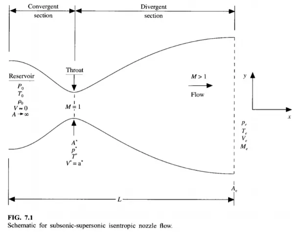
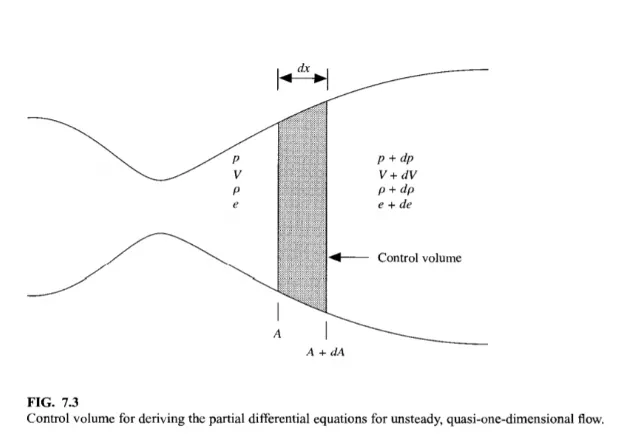
We assume that at a given section, where the cross section area is A, the flow properties are unifrom across the section. Hence, although the area of the nozzle changes as a function of distance along the nozzle,X, and therefore in reality the flow field is two dimensionalm We make the assumption that the flow properties vary only with X; this is tantamount to assuming uniform flow properties across any given cross-section. Such flow is defines as Quasi one dimensional flow.
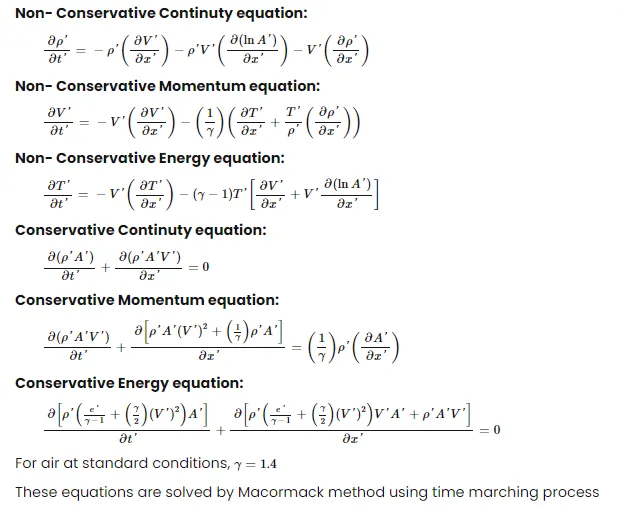
The governing continuit, momentum and enerygy equations in terms of non dimensional variables for this quasi one dimensional steady and isentropic flwo can be expressed respectively as
MacCarmack Method:
To discretize the numerical solution we use the technique called MacCarmack method. The MacCarmack method is a variation of the two-step Lax-Wendroff Scheme but is much simpler in application.
The application of Maccarmack method proceeds in two steps; a predictor step which is followed by a corrector step
Predictor Step: In the predictor step, a provisional value of u at time level n+1 is estimated obtained by replacing the spatial and temporal derivatives in the previous first order equation using Forward difference scheme Delta t is used for Timestep
Corrector Step: In the corrector step, the predicted value u^n+1 is corrected according to the equation. Note that the corrector step uses Backward difference scheme for spatial derivative. The time-step used in the corrector step is Delta T/2 in contrast to the Delta t used in the predictor step.
Main Program:
Matlab code with Explanation
close all
clc
L=3;
n=[31 62 93];
nt=1:1400;
cf1=0.5;
for i=1:length(n)
    x=linspace(0,L,n(i));
    [mfr_nc,mfr_throat_nc]=non_conservative(L,n(i),nt,cf1);
    [mfr_c,mfr_throat_c]=conservative(L,n(i),nt,cf1);
    figure(7)
    subplot(2,1,1)
    plot(nt,mfr_throat_c,'b',nt,mfr_throat_nc,'r','linewidth',1)
    xlabel('Time steps (nt)')
    ylabel('Mass flow rate')
    legend('Conservative Form','Non Conservative Form')
    title('Mass flow rate using Non Conservative Form vs Conservative Form at throat point i =16')
    subplot(2,1,2)
    plot(x,mfr_c,'b',x,mfr_nc,'r','linewidth',1)
    xlabel('Length of Nozzle')
    ylabel('Mass flow rate')
    legend('Conservative form','Non Conservative form')
    title('Mass flow rate using Non Conservative form vs Conservative From in the Nozzle')
    figure(8)
    subplot(2,1,1)
    plot(nt,mfr_throat_c,'linewidth',1)
    hold on
    xlabel('Time Steps (nt)')
    ylabel('Mss flow rate')
    legend('@31 Nodes','@62 Nodes','@93 Nodes')
    title('Conservative form: Grid Independency Test at throat point i=16')
    subplot(2,1,2)
    plot(nt,mfr_throat_nc,'linewidth',1)
    hold on
    xlabel('Time steps (nt)')
    ylabel('Mass flow rate')
    legend('@31 nodes','@62 nodes','@93 nodes')
    title('Non conservative form: Grid independency test at throat point i=16')
    figure(9)
    subplot(2,1,1)
    plot(x,mfr_c,'linewidth',1)
    hold on
    xlabel('Length of nozzle')
    ylabel('Mass flow rate')
    legend('@31 nodes','@62 nodes','@93 nodes')
    title('Conservative form: Grid independencyy test along the nozzle')
    subplot(2,1,2)
    plot(x,mfr_nc,'linewidth',1)
    hold on
    xlabel('Length of nozzle')
    ylabel('Mass flow rate')
    legend('@31 nodes','@62 nodes','@93 nodes')
    title('Non conservative form: Grid independency test along the nozzle')
end
Non Conservative Function
function[mfr_nc,mfr_throat_nc]=non_conservative(L,n,nt,cf1)
x=linspace(0,L,n);
dx=x(2)-x(1);
rho=1-0.3146*x;
T=1-0.2314*x;
v=(0.1+1.09*x).*T.^0.5;
a=1+2.2*(x-1.5).^2;
M=v./(T.^0.5);
mfr=rho.*a.*v;
p=rho.*T;
g=1.4;
for z=1:31
    u=(T(z))^(1/2);
    dt(z)= cf1*dx/(u + v(z));
end
dt=min(dt);
for i=1:length(nt)
    rho_old=rho;
    T_old=T;
    v_old=v;
    for j=2:n-1
        drho_dx=(rho(j+1)-rho(j))/dx;
        dv_dx=(v(j+1)-v(j))/dx;
        dT_dx=(T(j+1)-T(j))/dx;
        da_dx=(log(a(j+1))-log(a(j)))/dx;
        drho_dt_p(j)=-rho(j)*dv_dx-rho(j)*v(j)*da_dx-v(j)*drho_dx;
        dv_dt_p(j)=-v(j)*dv_dx-(1/g)*(dT_dx+(T(j)/rho(j))*drho_dx);
        dT_dt_p(j)=-v(j)*dT_dx-(g-1)*T(j)*(dv_dx+v(j)*da_dx);
        v(j)=v_old(j)+dv_dt_p(j)*dt;
        rho(j)=rho_old(j)+drho_dt_p(j)*dt;
        T(j)=T_old(j)+dT_dt_p(j)*dt;
        drho_dx=(rho(j)-rho(j-1))/dx;
        dv_dx=(v(j)-v(j-1))/dx;
        dT_dx=(T(j)-T(j-1))/dx;
        da_dx=(log(a(j))-log(a(j-1)))/dx;
        drho_dt_c(j)=-rho(j)*dv_dx-rho(j)*v(j)*da_dx-v(j)*drho_dx;
        dv_dt_c(j)=-v(j)*dv_dx-(1/g)*dT_dx+(T(j)/rho(j))*drho_dx;
        dT_dt_c(j)=-v(j)*dT_dx-(g-1)*T(j)*(dv_dx+v(j)*da_dx);
    end
    drho_dt_avg=0.5*(drho_dt_p+drho_dt_c);
    dv_dt_avg=0.5*(dv_dt_p+dv_dt_c);
    dT_dt_avg=0.5*(dT_dt_p + dT_dt_c);
    for k=2:n-1
        rho(k)=rho_old(k)+drho_dt_avg(k)*dt;
        v(k)=v_old(k)+dv_dt_avg(k)*dt;
        T(k)=T_old(k)+dT_dt_avg(k)*dt;
    end
    v(1)=2*v(2)-v(3);
    v(n)=2*v(n-1)-v(n-2);
    rho(n)=2*rho(n-1)-rho(n-2);
    T(n)=2*T(n-1)-T(n-2);
    p=rho.*T;
    M=v./T.^0.5;
    error(k)=abs(v(k)-v(k-1));
    mfr=rho.*a.*v;
    T_throat(i)=T(16);
    rho_throat(i)=rho(16);
    v_throat(i)=v(16);
    M_throat(i)=M(16);
    p_throat(i)=p(16);
    error_throat(i)=error(16);
    mfr_throat(i)=mfr(16);
    if n==31
        for ii=[1:50:201 700]
            if ii==i
                figure(1)
                plot(x,mfr,'linewidth',1)
                hold on
                title('Non-Conservative Form - Varioation of Mass flow rate distribution inside the nozzle at different time steps during the time-marching process ')
                xlabel('Length of nozzle')
                ylabel('Mass flow rate')
            elseif i==1400
                plot(x,mfr,'*r')
                legend('@1','@51','@101','@151','@201','@700','@1400')
            end
        end
    end
end
if n==31
    figure(2)
    plot(x,v,'b ',x,p,'r',x,T,'k',x,rho,'m',x,M,'g',x,mfr,'c')
    ylim([-0.1 3.7])
    title(sprintf('Timestep =%d',i))
    xlabel('Length of nozzle')
    ylabel('Non dimensional parameters')
    legend('Velocity','Pressure','Temperature','Density','Mach Number','Mass flow rate','Location','Northwest')
    title('Non Conservative form-Steady state distribution of primitive variables inside the nozzle')
figure(3)
plot(nt,rho_throat)
hold on
plot(nt,v_throat,'linewidth',1)
plot(nt,p_throat,'linewidth',1)
plot(nt,T_throat,'linewidth',1)
plot(nt,M_throat,'linewidth',1)
plot(nt,mfr_throat,'linewidth',1)
xlabel('Time steps(nt)')
ylabel('Non dimensional parameters')
legend('Density','Velocity','Pressure','Temperature','Mach Number','Mass flow rate')
title('Non conservative form-Time wise variation of the primitive variables at throat point i=16')
end
mfr_nc=mfr;
mfr_throat_nc=mfr_throat;
end
Conservative Function
function[mfr_c,mfr_throat_c]=conservative(L,n,nt,cf1)
x=linspace(0,L,n);
dx=x(2)-x(1);
for ii=1:length(x)
    if (x(ii)<=0.5)
        rho(ii)=1;
        T(ii)=1;
    elseif (x(ii)>0.5)&&(x(ii)<=1.5)
        rho(ii)=1-0.366*(x(ii)-0.5);
        T(ii)=1-0.167*(x(ii)-0.5);
    elseif (x(ii)>1.5)&&(x(ii)<=3.5)
        rho(ii)=0.634-0.3789*(x(ii)-1.5);
        T(ii)=0.833-0.3507*(x(ii)-1.5);
    end
end
a=1+2.2*(x-1.5).^2;
g=1.4;
u1=rho.*a;
u2=0.59*ones(1,n);
v=u2./u1;
u3=u1.*((T./(g-1))+(g/2).*v.^2);
M=v./(T.^0.5);
mfr=rho.*a.*v;
p=rho.*T;
for z=1:31
    u=(T(z))^(1/2);
    dt(z)=cf1*dx/(u+v(z));
end
dt=min(dt);
for i=1:length(nt)
    u1_old=u1;
    u2_old=u2;
    u3_old=u3;
    for j=2:n-1
        f1=u2;
        f2=((u2.^2)./u1)+((g-1)/g)*(u3-((g/2)*(u2.^2)./u1));
        f3=((g.*u2.*u3)./u1)-((g*(g-1)/2)*(u2.^3)./(u1.^2));
        j1=(1/g)*rho(j)*T(j)*((a(j+1)-a(j))/dx);
        du1_dt_p(j)=-(f1(j+1)-f1(j))/dx;
        du2_dt_p(j)=-(f2(j+1)-f2(j))/dx +j1;
        du3_dt_p(j)=-(f3(j+1)-f3(j))/dx;
        u1(j)=u1_old(j)+du1_dt_p(j)*dt;
        u2(j)=u2_old(j)+du2_dt_p(j)*dt;
        u3(j)=u3_old(j)+du3_dt_p(j)*dt;
        rho=u1./a;
        T=(g-1).*(u3./u1-(g/2).*(u2./u1).^2);
        f1=u2;
        f2=u2.^2./u1+((g-1)/g).*(u3-(g/2)*u2.^2./u1);
        f3=g.*u2.*u3./u1-0.5*g*(g-1).*u2.^3./u1.^2;
        j2=(1/g)*(rho(j)*T(j)*(a(j)-a(j-1))/dx);
        du1_dt_c(j)=-(f1(j)-f1(j-1))/dx;
        du2_dt_c(j)=-(f2(j)-f2(j-1))/dx +j2;
        du3_dt_c(j)=-(f3(j)-f3(j-1))/dx;
    end
    du1_dt_avg=0.5*(du1_dt_p+du1_dt_c);
    du2_dt_avg=0.5*(du2_dt_p+du2_dt_c);
    du3_dt_avg=0.5*(du3_dt_p+du3_dt_c);
    for k=2:n-1
        u1(k)=u1_old(k)+du1_dt_avg(k)*dt;
        u2(k)=u2_old(k)+du2_dt_avg(k)*dt;
        u3(k)=u3_old(k)+du3_dt_avg(k)*dt;
    end
    u1(1)=a(1);
    u2(1)=2*u2(2)-u2(3);
    u3(1)=u1(1)*(T(1)/(g-1)+(g*(u2(1)/u1(1))^2));
    u1(n)=2*u1(n-1)-u1(n-2);
    u2(n)=2*u2(n-1)-u3(n-2);
    u3(n)=2*u3(n-1)-u3(n-2);
    rho=u1./a;
    v=u2./u1;
    T=(g-1).*(u3./u1-(g/2).*(u2./u1).^2);
    p=rho.*T;
    M=v./T.^0.5;
    error(k)=abs(v(k)-v(k-1));
    mfr=u2;
    T_throat(i)=T(16);
    rho_throat(i)=rho(16);
    v_throat(i)=v(16);
    M_throat(i)=M(16);
    p_throat(i)=p(16);
    error_throat(i)=error(16);
    mfr_throat(i)=mfr(16);
    if n==31
        for ii=[1:50:201 700]
            if ii==i
                figure(4)
                plot(x,mfr,'linewidth',1)
                hold on
                title('Conservative Form- Variation of Mass flow rate distribution Inside the Nozzle at different time steps during the time-marching process')
                xlabel('Length of Nozzle')
                ylabel('Mass flow rate')
            elseif i==1400
                plot(x,mfr,'*r')
                legend('@1','@51','@101','@151','@201','@700','@1400')
            end
        end
    end
end
if n==31
    figure(5)
    plot(x,v,'b',x,p,'r',x,T,'k',x,rho,'m',x,M,'g',x,mfr,'c')
    ylim([-0.1 3.7])
    title(sprintf('Timestep=%d',i))
    xlabel('Length of nozzle')
    ylabel('Non dimensional parameters')
    legend('Velocity','Pressure','Temperature','Density','Mach Number','Mass flow rate','Location','Northwest')
    title('Conservative Form-Steady-State distribution of primitive variables inside the nozzle')
    figure(6)
    plot(nt,rho_throat)
    hold on
    plot(nt,v_throat,'linewidth',1)
    plot(nt,p_throat,'linewidth',1)
    plot(nt,T_throat,'linewidth',1)
    plot(nt,M_throat,'linewidth',1)
    plot(nt,mfr_throat,'Linewidth',1)
    xlabel('Timesteps (nt)')
    ylabel('Non Dimensional Parameters')
    legend('Density','Velocity','Pressure','Temperature','Mach Number','Mass flow rate')
    title('COnservative Form-Time wise variation of the primitive variables at throat point i=16')
end
mfr_c=mfr;
mfr_throat_c=mfr_throat;
end
Results
Non Conservative Form
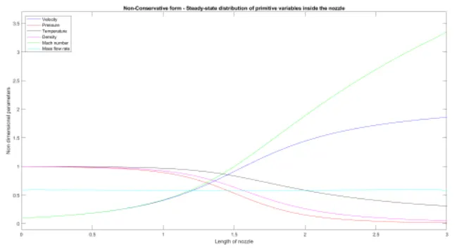
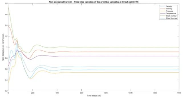
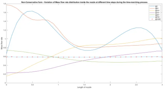
Figure 1 Steady state distribution of non dimensional primitive variables at the end of time step.
Figure 2 shows Time wise variation of primitive variables at throat point i=16 around the time step of 500 the flow field variables obtained stabled solution
Figure 3 shows the variation of mass flow rate distribution inside the nozzle at different time steps during the time marching process. The mass flow rate finally settled at 0.58.
Conservative Form:
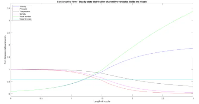
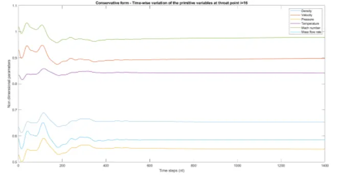
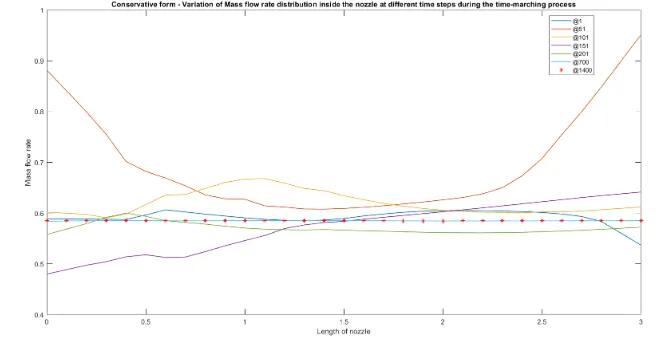
Figure 1 Steady state distribution of non dimensional primitive variables at the end of time step.
Figure 2 shows Time wise variation of primitive variables at throat point i=16 around the time step of 600 the flow field variables obtained stabled solution
Figure 3 shows the variation of mass flow rate distribution inside the nozzle at different time steps during the time marching process. The mass flow rate finally settled at 0.56.
Non-Conservative Form vs Conservative Form
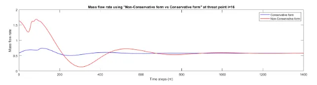
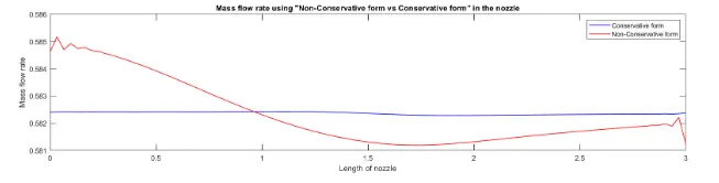
Figure shows the comparios of mass flow rate using both conservative and non conservative forms
In 1 Both the forms reached the stable and exact solution by the end of the time steps. But conservative form obtained the stability at lesser time steps
In 2 The difference between both the forms is very less in the nozzle. But the mass flow rate in the conservative form is constant where as in non conservative form it is varying with 0.52+_ 0.003.
Grid Independency test for both Non Conservative and Conservative Form:
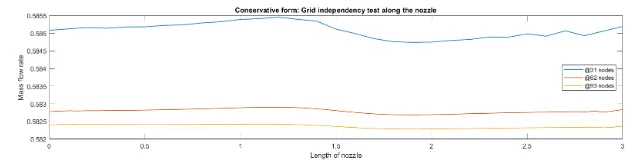
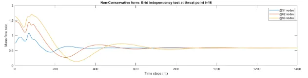
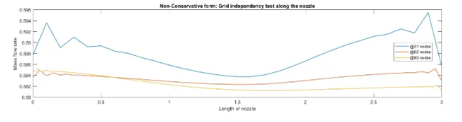
Figure shows the Gird Independance test in both the forms
Mass Flow rate varying with time step at throat point
At 3 different grid sizes, though the values are different at the starting of time marching process the solution obtained is stable and almost same by the end of time marching
The solution obtained using 3 different grid sizes resulting 3 different solutions within the range of 0.589+-0.006. the difference between them is very small which can be neglect/ignored.
We can conclude that the plot is not much changing when the number of grid points are doubled up and nearly tripled up. Although there is a slight change at the throat area alone in the conservation form, which is not considerably significant.