Week 7 - Simulation of a 1D Super-sonic nozzle flow simulation using Macormack Method

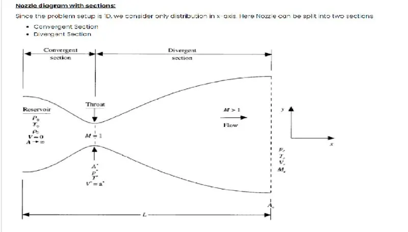
Simulation of 1D supersonic nozzle flow using Macormack method:

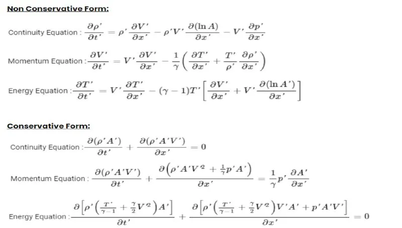
To discretize the equation by using the Macormack method. In this technique, there are two different methods

1. Predictor method

2. Corrector method

procedure;

coding is started by giving the required inputs like no of nodes, time step 'dt', pressure, density, velocity, and temperature for both conservative and non-conservative equations.

and tic toc commands are used for time elapsed in functions

and plot the required variable for getting the results

close all
clear all
clc

% inputs
n = 31;
x = linspace(0,3,n);
dx = x(2)-x(1);
gamma = 1.4;
nt = 1400;
%courant number
c = 0.5;

% tic;
[mass_flow_rate, presure, mach_number, rho_Nc, v_Nc, t_Nc, rho_inside, v_inside, t_inside, mass_flow_inside, presure_inside, mach_inside] = non_conservative_equations(x, dx, n, gamma,nt,c);
time_taken_Nc = toc;

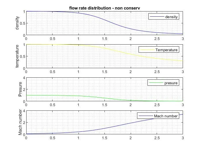
figure(2)
 % Density
 subplot(4,1,1)
 plot(x,rho_Nc,'Color','b')
 ylabel('density')
 legend({'density'});
 axis([0 3 0 1])
 title('flow rate distribution - non conserv')
 grid minor;

 %Temparature
 subplot(4,1,2)
 plot(x,t_Nc,'Color','y')
 ylabel('temperature')
 legend({'Temperature'});
 axis([0 3 0 1])
 grid minor;
 
  %Presure
 subplot(4,1,3)
 plot(x,presure,'Color','g')
 ylabel('Presure')
 legend({'presure'});
 axis([0 3 0 4])
 grid minor;

 %Mach number
 subplot(4,1,4)
 plot(x,mach_number,'Color','b')
 ylabel('Mach number')
 legend({'Mach number'});
 axis([0 3 0 4])
 grid minor;

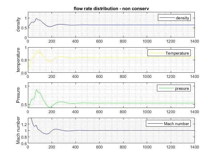
 figure(3)
 % Time variation at inside area or throat 

 % Density
 subplot(4,1,1)
 plot(linspace(1,nt,nt),rho_inside,'Color','b')
 ylabel('density')
 legend({'density'});
 axis([0 1400 0 1.3])
 title('flow rate distribution - non conserv')
 grid minor;

 %Temparature
 subplot(4,1,2)
 plot(linspace(1,nt,nt),t_inside,'Color','y')
 ylabel('temperature')
 legend({'Temperature'});
 axis([0 1400 0.6 1])
 grid minor;
 
  %Presure
 subplot(4,1,3)
 plot(linspace(1,nt,nt),presure_inside,'Color','g')
 ylabel('Presure')
 legend({'presure'});
 axis([0 1400 0.4 1.1])
 grid minor;

 %Mach number
 subplot(4,1,4)
 plot(linspace(1,nt,nt),mach_inside,'Color','b')
 ylabel('Mach number')
 legend({'Mach number'});
 axis([0 1400 0.6 1.4])
 grid minor;

%function file of Non-conservative equations

function [mass_flow_rate, presure, mach_number, rho_Nc, v_Nc, t_Nc, rho_inside, v_inside, t_inside, mass_flow_inside, presure_inside, mach_inside] = non_conservative_equations(x, dx, n, gamma,nt,c)

% calculate initial profiles

rho_Nc = 1-0.3146.*x;
t_Nc = 1-0.2341.*x;
v_Nc = (0.1+1.09*x).*t_Nc.^0.5;

% Area
a = 1+2.2*(x-1.5).^2;

% Throat
throat = find(a==1);


% time step
dt =min(c.*dx./(sqrt(t_Nc)+v_Nc));

for k =1:nt

    % udating old values
    rho_old = rho_Nc;
    t_old = t_Nc;
    v_old = v_Nc;

    % predictor method

    for j = 2:n-1

        dvdx = (v_Nc(j+1)-v_Nc(j))/dx;
        drhodx = (rho_Nc(j+1)-rho_Nc(j))/dx;
        dtdx = (t_Nc(j+1)-t_Nc(j))/dx;
        dlogadx = (log(a(j+1))-log(a(j)))/dx;

        % continuty equation
        drhodt_p(j) = -rho_Nc(j)*dvdx-rho_Nc(j)*v_Nc(j)*dlogadx-v_Nc(j)*drhodx;

        % momentum quation
        dvdt_p(j) = -v_Nc(j)*(dvdx)-(1/gamma)*(dtdx+(t_Nc(j)/rho_Nc(j))*drhodx);

        % energy quation
        dtdt_p(j) = -v_Nc(j)*(dtdx)-(gamma-1)*t_Nc(j)*(dvdx+v_Nc(j)*dlogadx);

        % solution update
        v_Nc(j) = v_Nc(j) + dvdt_p(j)*dt;
        rho_Nc(j) = rho_Nc(j) + drhodt_p(j)*dt;
        t_Nc(j) = t_Nc(j) + dtdt_p(j)*dt;

    end

    % corrector method

    for j = 2:n-1

        dvdx = (v_Nc(j)-v_Nc(j-1))/dx;
        drhodx = (rho_Nc(j)-rho_Nc(j-1))/dx;
        dtdx = (t_Nc(j)-t_Nc(j-1))/dx;
        dlogadx = (log(a(j))-log(a(j-1)))/dx;

        % continuty equation
        drhodt_c(j) = -rho_Nc(j)*dvdx-rho_Nc(j)*v_Nc(j)*dlogadx-v_Nc(j)*drhodx;

        % momentum quation
        dvdt_c(j) = -v_Nc(j)*(dvdx)-(1/gamma)*(dtdx+(t_Nc(j)/rho_Nc(j))*drhodx);

        % energy quation
        dtdt_c(j) = -v_Nc(j)*(dtdx)-(gamma-1)*t_Nc(j)*(dvdx+v_Nc(j)*dlogadx);

    end
    % compute the average time derivative
    drhodt = 0.5*(drhodt_p+drhodt_c);
    dvdt = 0.5*(dvdt_p+dvdt_c);
    dtdt = 0.5*(dtdt_p+dtdt_c);

    % final solution update

    for i=2:n-1
        rho_Nc(i) = rho_old(i)+drhodt(i)*dt;
        v_Nc(i) = v_old(i)+dvdt(i)*dt;
        t_Nc(i) = t_old(i)+dtdt(i)*dt;
    end

    % boundary condition
    % inlet
    v_Nc(1) = 2*v_Nc(2)-v_Nc(3);

    % outlet
    v_Nc(n) = 2*v_Nc(n-1)-v_Nc(n-2);
    rho_Nc(n) = 2*rho_Nc(n-1)-rho_Nc(n-2);
    t_Nc(n) = 2*t_Nc(n-1)-t_Nc(n-2);

    % physical properties
    mass_flow_rate = rho_Nc.*a.*v_Nc;
    presure = rho_Nc.*t_Nc;
    mach_number = (v_Nc./sqrt(t_Nc));

    %inside variables at throat area
    rho_inside(k) = rho_Nc(throat);
    t_inside(k) = t_Nc(throat);
    v_inside(k) = v_Nc(throat);
    mass_flow_inside(k) = mass_flow_rate(throat);
    presure_inside(k) = presure(throat);
    mach_inside(k) = mach_number(throat);


    % mass flow rate at different time steps
    figure(1)
    if k == 50
        plot(x, mass_flow_rate,'m','LineWidth',1.25)
        hold on
    elseif k == 100
        plot(x, mass_flow_rate,'c','linewidth', 1)
        hold on
    elseif k == 200
        plot(x, mass_flow_rate,'Y','linewidth', 0.5)
    end
    axis([0 3 0 2])
    xlabel('Distance')
    ylabel('mass_flow_rate')
    title(' Mass flow rate at diff time step-non conv equs')
end
end


% Conservation equations

tic;
[mass_flow_rate_c, pressure_c, mach_number_c, rho_c, v_c, t_c, rho_inside_c, v_inside_c, t_inside_c, mass_flow_inside_c, pressure_inside_c, mach_inside_c] = conservative_equations(x, dx, n, gamma,nt,c);
time_taken_Nc = toc;

%Density at throat
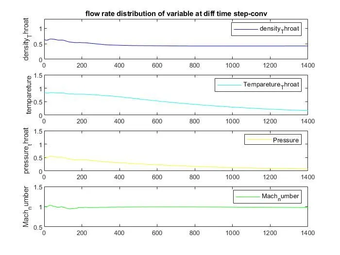
figure(5)
subplot(4,1,1)
plot(rho_inside_c,'color','b')
ylabel('density_Throat')
legend({'density_Throat'})
axis([0 1400 0 1.3])
title('flow rate distribution of variable at diff time step-conv')
 
%Tempareture at thraot
subplot(4,1,2)
plot(t_inside_c,'color','c')
ylabel('tempareture')
legend({'Tempareture_Throat'})
axis([0 1400 0 1.5])

%Pressure at throat
subplot(4,1,3)
plot(pressure_inside_c,'color','y')
ylabel('pressure_throat')
legend({'Pressure'})
axis([0 1400 0 1.5])

%Mach number at throat
subplot(4,1,4)
plot(mach_inside_c,'color','g')
ylabel('Mach_number')
legend({'Mach_number'})
axis([0 1400 0.5 1.5])


%Density
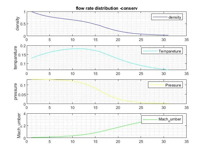
figure(6)
subplot(4,1,1)
plot(rho_c,'color','b')
ylabel('density')
legend({'density'})
title('flow rate distribution -conserv')
grid minor;

%Tempareture  
subplot(4,1,2)
plot(t_c,'color','c')
ylabel('tempareture')
legend({'Tempareture'})
grid minor;


% pressure
subplot(4,1,3)
plot(pressure_c,'color','y')
ylabel('pressure')
legend({'Pressure'})
grid minor;

% mach number
subplot(4,1,4)
plot(mach_number_c,'color','g')
ylabel('Mach_number')
legend({'Mach_number'})
grid minor;

% Function file for Conservative equations


function [mass_flow_rate_c, pressure_c, mach_number_c, rho_c, v_c, t_c, rho_inside_c, v_inside_c, t_inside_c, mass_flow_inside_c, pressure_inside_c, mach_inside_c] = conservative_equations(x, dx, n, gamma,nt,c)

% intial comditions
for i = 1:n
    if x(i)>=0 && x(i)<=0.5
        rho_c(i) = 1;
        t_c(i) = 1;
    elseif x(i)>=0.5 && x(i)<=1.5
        rho_c(i) = 1-0.366*(x(i)-0.5);
        t_c(i) = 1-0.167*(x(i)-0.5);
    elseif x(i)>=1.5 && x(i)<=3
        rho_c(i) = 0.634-0.3879*(x(i)-1.5);
        t_c(i) = 0.833-0.3507*(x(i)-1.5) ;
    end
end

% Area
a = 1+2.2*(x-1.5).^2;

% Throat
throat = find(a==1);

% initial values for velocity and pressure
v_c = 0.59./(rho_c.*a);
pressure_c = rho_c.*t_c;

% intial conditions
u1 =rho_c.*a;
u2 = rho_c.*a.*v_c;
u3 = rho_c.*a.*((t_c./(gamma-1))+(gamma/2).*v_c.^2);

%time loop
for k= 1:nt

    % time step
    dt = min(c.*dx./(sqrt(t_c)+v_c));

    % copy of old values
    u1_old = u1;
    u2_old = u2;
    u3_old = u3;

    % flex
    f1 = u2;
    f2 =(u2.^2./u1)+((gamma-1)/gamma)*(u3-((gamma/2)*(u2.^2)./u1));
    f3 = ((gamma*u2.*u3)./u1)-((gamma*(gamma-1)/2) * (u2.^3)./(u1.^2));


    %predictor method
    for m = 2:n-1

        % main equation
        j_2(m) = (1/gamma)*rho_c(m)*t_c(m)*((a(m+1)-a(m))/dx);

        % continuity equation
        du1dt_p(m) = -((f1(m+1)-f1(m))/dx);

        % momentum equation
        du2dt_p(m) = -((f2(m+1)-f2(m))/dx)+j_2(m);

        % energy equation
        du3dt_p(m) = -((f3(m+1)-f3(m))/dx);

        % solution updates

        u1(m) = u1(m)+du1dt_p(m)*dt;
        u2(m) = u2(m)+du2dt_p(m) *dt;
        u3(m) = u3(m)+du3dt_p(m)*dt;


    end
    rho_c = (u1./a);
    v_c = (u2./u1);
    t_c = (gamma-1)*(u3./u1-(gamma/2).*v_c.^2);

    %corrector method

    % flex
    f1 = u2;
    f2 =(u2.^2./u1)+((gamma-1)/gamma)*(u3-((gamma/2)*(u2.^2)./u1));
    f3 = ((gamma*u2.*u3)./u1)-((gamma*(gamma-1)/2) * (u2.^3)./(u1.^2));

    for m = 2:n-1

        % main euation
        j_2(m) = (1/gamma)*rho_c(m)*t_c(m)*((a(m)-a(m-1))/dx);

        % special terms
        du1dt_c(m) = -((f1(m)-f1(m-1))/dx);
        du2dt_c(m )= -(f2(m)-f2(m-1))/dx+j_2(m);
        du3dt_c(m) = -((f3(m)-f3(m-1))/dx);

    end

    % compute time dervative
    du1dt = 0.5*(du1dt_c+du1dt_p);
    du2dt = 0.5*(du2dt_c+du2dt_p);
    du3dt = 0.5*(du3dt_c+du3dt_p);

    % solution update
    for i = 2:n-1
        u1(i) = u1_old(i)+du1dt(i)*dt;
        u2(i) = u2_old(i)+du2dt(i)*dt;
        u3(i) = u3_old(i)+du3dt(i)*dt;
    end

    % applyng boundry conditions
    
    % inlet
    u1(1) = rho_c(1)*a(1);
    u2(1) = 2*u2(2)-u2(3);
    v_c(1)= u2(1)./u1(1);
    u3(1) = u1(1)*(t_c(1)/(gamma-1))+((gamma/2)*(v_c(1)).^2);

    % out let
    u1(n) = 2*u1(n-1)-u1(n-2);
    u2(n) = 2*u2(n-1)-u2(n-2);
    u3(n) = 2*u3(n-1)-u3(n-2);

    rho_c = u1./a;
    v_c = (u2./u1);
    t_c = (gamma-1).*((u3./u1)-((gamma/2).*v_c.^2));
    pressure_c = rho_c.*t_c;

    % primetive values
    mass_flow_rate_c = rho_c.*a.*v_c;
    pressure_c = rho_c.*t_c;
    mach_number_c = (v_c./sqrt(t_c));

    %inside variables at throat area

    rho_inside_c(k) = rho_c(throat);
    t_inside_c(k) = t_c(throat);
    v_inside_c(k) = v_c(throat);
    mass_flow_inside_c(k) = mass_flow_rate_c(throat);
    pressure_inside_c(k) = pressure_c(throat);
    mach_inside_c(k) = mach_number_c(throat);



%     mass flow rate at different time steps
    figure(4)
    if k == 50
        plot(x, mass_flow_rate_c,'m','LineWidth',1.25)
        hold on
    elseif k == 100
        plot(x, mass_flow_rate_c,'c','linewidth', 1)
        hold on
    elseif k == 200
        plot(x, mass_flow_rate_c,'Y','linewidth', 0.5)
    end
    axis([0 3 0 1])
    xlabel('Distance')
    ylabel('mass_flow_rate_c')
    title('Mass flow rate at diff time step - conv equs')
end
end

Conclusion

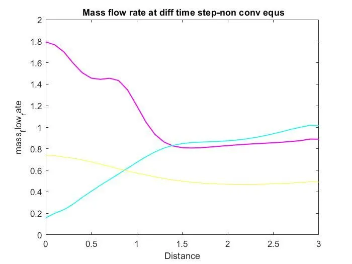
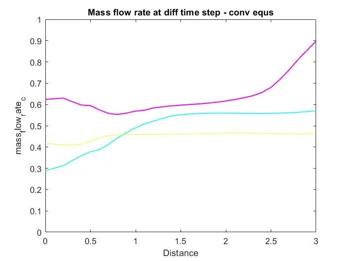
In these pictures, we can say that values are slightly different for both conservative and non-conservative equations.

But conservative equations are faster than non-conservative questions and if grid points are more solutions would not be faster so solution depends on the no of grid points also.