Week 11 - Simulation of Flow through a pipe in OpenFoam

Simulation of Flow through a pipe in OpenFoam

Aim:

1 creating the block mesh for the wedge according to requirements by using Matlab

2 Select the icoFoam solver to solve the flow through pipe in OpenFoam

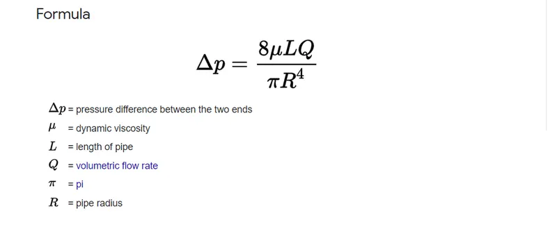
3 Post process the velocity profile and shear stress and compare the simulation results with analytical results obtained using the Hagen-Poiseuille equation.

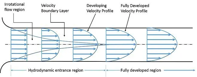
Hydrodynamic Length(Le):

The hydrodynamic entry length is the point at which the velocity profile is fully developed in the tube from the point of entry for the fluid. The thermal entry length is the point at which the temperature profile is fully developed from the point at which the tube wall is heated or cooled.

Variables:

Dia = 0.004;

Radius(r) = 0.002;

Radial distance = 0 to r;

Dinamic viscocity mu = 0.000083 N/m^2;

Density(nu) = 997kg/m^3;

Reynaulds number = 2100;

Matlab Program for creating blockmesh

close all
clear all
clc

f1 = fopen("blockMeshDict","w")
h1="/*--------------------------------*- C++ -*----------------------------------*\";
h2="| ========= | |";
h3="| \\ / F ield | OpenFOAM: The Open Source CFD Toolbox |";
h4="| \\ / O peration | Version: 4.0 |";
h5="| \\ / A nd | Web: www.OpenFOAM.org |";
h6="| \\/ M anipulation | |";
h7="\*---------------------------------------------------------------------------*/";

h = "FoamFile";
h8 = "{";
 h9 ="version 2.0;";
 h10 = "format      ascii;";
 h11 = "class dictionary";
 h12 = "object blockMeshDict";
h13 = "}";
h14 = "// * * * * * * * * * * * * * * * * * * * * * * * * * * * * * * * * * * * * * //";


fprintf(f1,"%s \n",h1);
fprintf(f1,"%s \n",h2);
fprintf(f1,"%s \n",h3);
fprintf(f1,"%s \n",h4);
fprintf(f1,"%s \n",h5);
fprintf(f1,"%s \n",h6);
fprintf(f1,"%s \n",h7);
fprintf(f1,"%s \n",h);
fprintf(f1,"%s \n",h8);
fprintf(f1,"%s \n",h9);
fprintf(f1,"%s \n",h10);
fprintf(f1,"%s \n",h11);
fprintf(f1,"%s \n",h12);
fprintf(f1,"%s \n",h13);
fprintf(f1,"%s \n",h14);

con = "convertToMeters 1;";
ver = "vertices";

fprintf(f1,"%s \n",con);
fprintf(f1,"%s \n",ver);

s1 = blanks(4);
s2 = blanks(8);
s3 = blanks(12);

r = 0.01;
theta = 3; % in degres


v0 = [0 0 0];
v1 = [0 r*cosd(theta/2) r*sind(theta/2)];
v2 = [0 r*cosd(theta/2) -r*sind(theta/2)];
v3 = [1 0 0];
v4 = [1 r*cosd(theta/2) r*sind(theta/2)];
v5 = [1 r*cosd(theta/2) -r*sind(theta/2)];



fprintf(f1,"%s \n","(");
fprintf(f1,"%s (%d %d %d)\n",s1,v0);
fprintf(f1,"%s (%d %d %d)\n",s1,0,r*cosd(theta/2),r*sind(theta/2));
fprintf(f1,"%s (%d %d %d)\n",s1,v2);
fprintf(f1,"%s (%d %d %d)\n",s1,v3);
fprintf(f1,"%s (%d %d %d)\n",s1,v4);
fprintf(f1,"%s (%d %d %d)\n",s1,v5);
fprintf(f1,"%s \n",");");

fprintf(f1,"%s \n","blocks");

fprintf(f1,"%s \n","(");
fprintf(f1,"%s hex (0 3 5 2 0 3 4 1)(%d %d %d) SimpleGrading (%d %d %d)\n",s1,300,30,1,1,0.1,1);
fprintf(f1,"%s \n",s1,");");

fprintf(f1,"%s \n",s1,"edges");
fprintf(f1,"%s \n",s1,"(");
fprintf(f1,"%s arc 1 2 (%d %d %d)\n",s1,1,0.2,1);
fprintf(f1,"%s arc 4 5 (%d %d %d)\n",s1,1.2,2,0);
fprintf(f1,"%s \n",s1,");");
fprintf(f1,"%s \n",s1,"boundary");
fprintf(f1, 'boundary\n');
fprintf(f1, '(\n');
fprintf(f1, '\t inlet \n');
fprintf(f1, '\t {\n');
fprintf(f1, '\t\t type patch;\n');
fprintf(f1, '\t\t faces\n');
fprintf(f1, '\t\t (\n');
fprintf(f1, '\t\t\t (0 1 2 0)\n');
fprintf(f1, '\t\t );\n');
fprintf(f1, '\t }\n');

fprintf(f1, '\t outlet\n');
fprintf(f1, '\t {\n');
fprintf(f1, '\t\t type patch;\n');
fprintf(f1, '\t\t faces\n');
fprintf(f1, '\t\t (\n');
fprintf(f1, '\t\t\t (3 5 4 3)\n');
fprintf(f1, '\t\t );\n');
fprintf(f1, '\t }\n');

fprintf(f1, '\t top\n');
fprintf(f1, '\t {\n');
fprintf(f1, '\t\t type wall;\n');
fprintf(f1, '\t\t faces\n');
fprintf(f1, '\t\t (\n');
fprintf(f1, '\t\t\t (1 4 5 2)\n');
fprintf(f1, '\t\t );\n');
fprintf(f1, '\t }\n');

fprintf(f1, '\t front\n');
fprintf(f1, '\t {\n');
fprintf(f1, '\t\t type wedge;\n');
fprintf(f1, '\t\t faces\n');
fprintf(f1, '\t\t (\n');
fprintf(f1, '\t\t\t (0 3 4 1)\n');
fprintf(f1, '\t\t );\n');
fprintf(f1, '\t }\n');

fprintf(f1, '\t back\n');
fprintf(f1, '\t {\n');
fprintf(f1, '\t\t type wedge;\n');
fprintf(f1, '\t\t faces\n');
fprintf(f1, '\t\t (\n');
fprintf(f1, '\t\t\t (0 2 5 3)\n');
fprintf(f1, '\t\t );\n');
fprintf(f1, '\t }\n');

fprintf(f1, '\t axis\n');
fprintf(f1, '\t {\n');
fprintf(f1, '\t\t type empty;\n');
fprintf(f1, '\t\t faces\n');
fprintf(f1, '\t\t (\n');
fprintf(f1, '\t\t\t (0 3 3 0)\n');
fprintf(f1, '\t\t );\n');
fprintf(f1, '\t }\n');
fprintf(f1, '); \n\n');
fprintf(f1, 'mergePatchPairs\n');
fprintf(f1, '(\n');
fprintf(f1, ');\n');
header15='// * * * * * * * * * * * * * * * * * * * * * * * * * * * * * * * * * * * * * //'
fprintf(f1, '%s\n',header15);
fclose(f1);

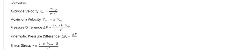
Analytical analysis for finding Shear stress:

close all
clear all
clc

% inputs 

% Reynaulds number
re = 2100;

% Diameter of the pipe in meters
d = 0.004;

% Dynamic viscosity
nu = 0.000889;

% Density
rho = 997;

% hydrodynamic length
le = 0.06*re*d;

%length of the pipe
L = le+0.7;

% radial distance
R = linspace(-0.01,0.01,1000);


% Hagen-poiseuille laws 

velocity_avg = (re*nu)/(rho*d);

velocity_max = 2*velocity_avg;

del_P = (8*nu*L*velocity_avg)/(d/2)^2;

del_Pk = (del_P/rho);

% calculation of shear stress

for i = 1:length(R)

tow(i) = 2*nu*velocity_max*(abs(R(i)))/(d/2)^2
end 

plot(R,tow)
xlabel('Radius')
ylabel('shear_stress')
legend('Shere_stress')
grid on

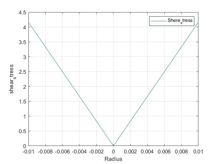
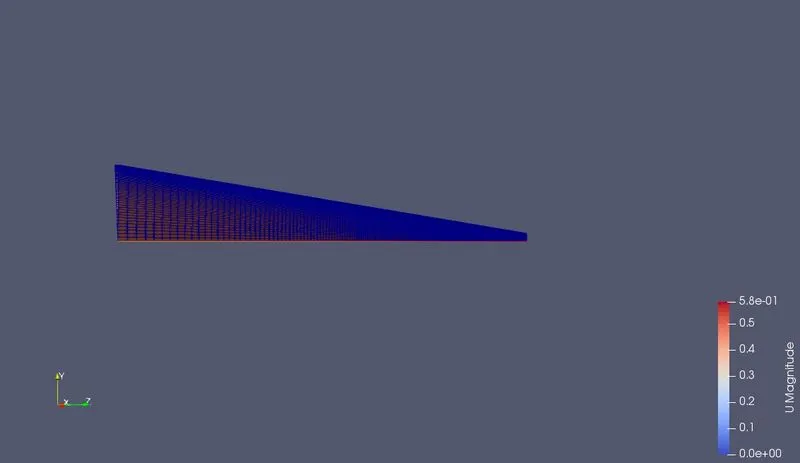
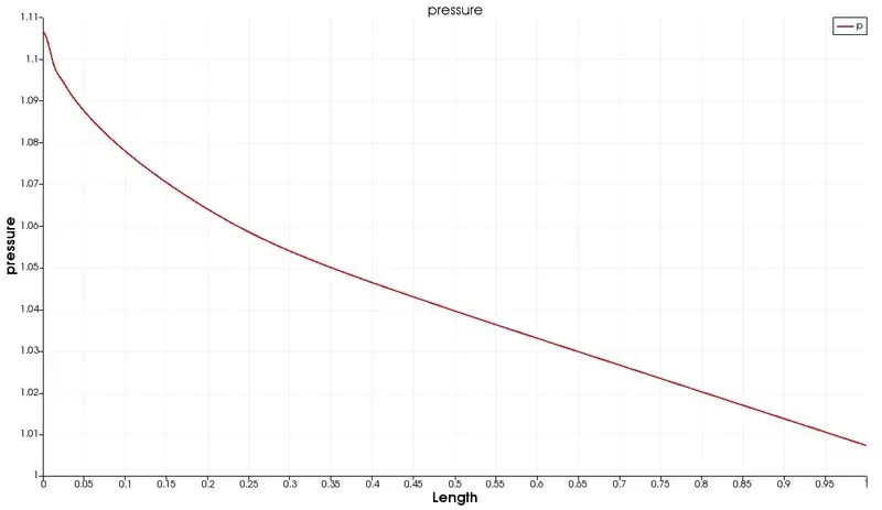
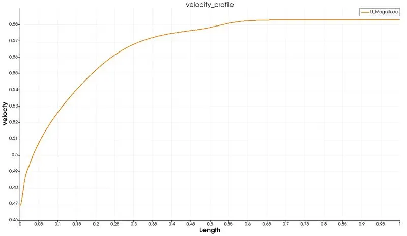
At point 0.5 in the graph, the velocity becomes stable

And the hydrodynamic length is 0.5 meters