Week 7 - Simulation of a 1D Super-sonic nozzle flow simulation using Macormack Method
Supersonic quasi 2D nozzle flow using Maccomark’s method
Supersonic flow is the flow in which the Mach number is greater than one (speed of the object is greater than the speed of sound).
Maccomark’s method denotes explicit finite-difference technique which is second-order-accurate in both space and time.
It subdivides into two steps predictor step and corrector step.
The velocity components for the next time step can be calculated with second-order accuracy without using second order derivative
It consists of forward difference on the predictor and backward difference on the corrector and hence it is referred to as second-order accurate method.
Schematic representation of convergent-divergent sections of nozzle
The convergent-divergent nozzle device is used to accelerate the fluid speed that will come out of the nozzle. Let the reservoir section be the inlet condition where the flow speed is lesser as the area tends to infinity. Here the Mach number is less than one. At the nozzle let’s take the Mach number as one in which the flow speed is assumed to be equal to the speed of sound.
The area function for nozzle flow is given as
a = 1+2.2(x-1.5)2 for 0<= x <=3
Governing equations:
For non-conservative form
Continuity equations:
= -ρ’ - ρ’V’ - V’
Momentum equation:
= -V’ - [ + ]
Energy equations:
= -V’ - ( [ + V’ ]
The initial conditions:
ρ' at t = 0 = 1 -0.3146x’
V' at t = 0 = (0.1+1.09x’)
T' at t = 0 = 1 -0.2314x’
For conservative form
Continuity equations:
+ = 0
Momentum equation:
+ =
Energy equations:
+ = 0
Conditions for conservative form:
U1 =
U2= V’
U3 =
F1= V’=U2
F2= + V’
J2 =
Initial conditions:
ρ' at t = 0 = 1 (0<= x’ ,0.5)
= 1 -0.336 (x’ -0.5) (0.5<= x’ <1.5)
=(0.634 -0.3879(x’-1.5)) (1.5<=x’<3)
V' at t = 0 =
T' at t = 0 = 1 (0<= x’ ,0.5)
= (1-0.167(x’0.5)) (0.5<= x’ <1.5)
= (0.833 -0.3507(x’-1.5) (1.5<= x’ <=3)
Code for non-conservative form:
clc
close all
clear all
%inputs
n=31;
x=linspace(0,3,n);
dx=x(2)-x(1);
gamma=1.4;
th=round(n/2);
%calculate intital profile
rho=1-0.3146*x;
t= 1-0.2314*x;
v=(0.1+1.09*x).*t.^0.5;
%area
a=1+2.2*(x-1.5).^2;
%time step
nt=1400;
dt=min(0.5*dx./(sqrt(t)+v));
cfl=max((v+sqrt(t))*dt/dx);
%outer time loop
for k=1:nt
%predictor method
rho_old=rho;
v_old=v;
t_old=t;
for j=2:n-1
dvdx=(v(j+1)-v(j))/dx;
drhodx=(rho(j+1)-rho(j))/dx;
dtdx=(t(j+1)-t(j))/dx;
dlogadx=(log(a(j+1))-log(a(j)))/dx;
%continuity equation
drhodt_p(j)=-rho(j)*dvdx-rho(j)*v(j)*dlogadx-v(j)*drhodx;
%momentum equation
dvdt_p(j)= -v(j)*dvdx-(1/gamma)*(dtdx+(t(j)/rho(j))*drhodx);
%energy equation
dtdt_p(j)=-v(j)*dtdx-(gamma-1)*t(j)*(dvdx+v(j)*dlogadx);
%solution update
rho(j)=rho(j)+drhodt_p(j)*dt;
v(j)=v(j)+dvdt_p(j)*dt;
t(j)=t(j)+dtdt_p(j)*dt;
end
%corrrector method
for l=2:n-1
dvdx=(v(l)-v(l-1))/dx;
drhodx=(rho(l)-rho(l-1))/dx;
dtdx=(t(l)-t(l-1))/dx;
dlogadx=(log(a(l))-log(a(l-1)))/dx;
%continuity equation
drhodt_c(l)=-rho(l)*dvdx-rho(l)*v(l)*dlogadx-v(l)*drhodx;
%momentum equation
dvdt_c(l)= -v(l)*dvdx-(1/gamma)*(dtdx+(t(l)/rho(l))*drhodx);
%energy equation
dtdt_c(l)=-v(l)*dtdx-(gamma-1)*t(l)*(dvdx+v(l)*dlogadx);
end
%compute average time derivative
drhodt=0.5*(drhodt_p+drhodt_c);
dvdt=0.5*(dvdt_p+dvdt_c);
dtdt=0.5*(dtdt_p+dtdt_c);
for i=2:n-1
%solution update
rho(i)=rho_old(i)+drhodt(i)*dt;
v(i)=v_old(i)+dvdt(i)*dt;
t(i)=t_old(i)+dtdt(i)*dt;
end
%BC
%inlet
v(1)=2*v(2)-v(3);
%outlet
v(n)=2*v(n-1)-v(n-2);
rho(n)=2*rho(n-1)-rho(n-2);
t(n)=2*t(n-1)-t(n-2);
p=rho.*t; %pressure
M=v./sqrt(t); %Mach number
m=rho.*a.*v; %mass flow rate
hold on
if k==1
figure(3)
plot(x,m);
hold on
end
if k==50
figure(3)
plot(x,m);
hold on
end
if k==250
figure(3)
plot(x,m);
hold on
end
if k==500
figure(3)
plot(x,m);
hold on
end
if k==750
figure(3)
plot(x,m);
hold on
end
if k==1400
figure(3)
plot(x,m);
hold on
xlabel('Nozzle length')
ylabel('Mass flow rate')
title("Variation of Mass flow rate at nozzle for different time steps")
legend('1dt','50dt','250dt','500dt','750dt','1400dt')
end
end
% pause(0.003)
figure(1)
subplot(5,1,1)
plot(x,v)
xlabel('Nozzle length')
ylabel('Velocity')
title("Variation of velocity at nozzle")
subplot(5,1,2)
plot(x,rho)
xlabel('Nozzle length')
ylabel('Density')
title("Variation of density at nozzle")
subplot(5,1,3)
plot(x,t)
xlabel('Nozzle length')
ylabel('Temperature')
title("Variation of temperature at nozzle")
subplot(5,1,4)
plot(x,p)
xlabel('Nozzle length')
ylabel('Pressure')
title("Variation of pressure at nozzle")
subplot(5,1,5)
plot(x,M)
xlabel('Nozzle length')
ylabel('Mach Number')
title("Variation of Mach Number at nozzle")
figure(2)
plot(x,m)
xlabel('Nozzle length')
ylabel('Mass flow rate')
title("Variation of Mass flow rate at nozzle")
Plot results:
Flow parameters at nozzle
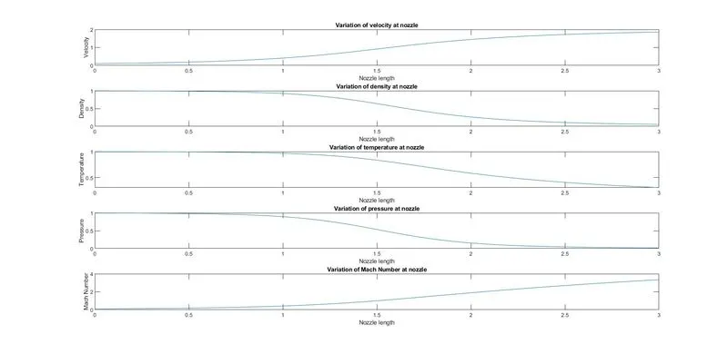
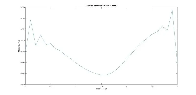
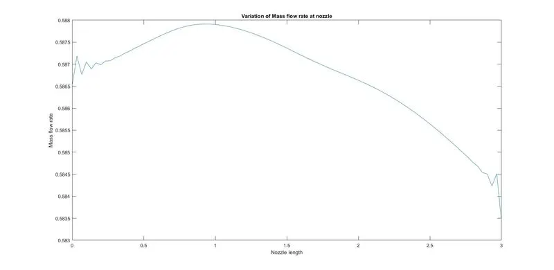
Mass flow rate at nozzle
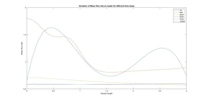
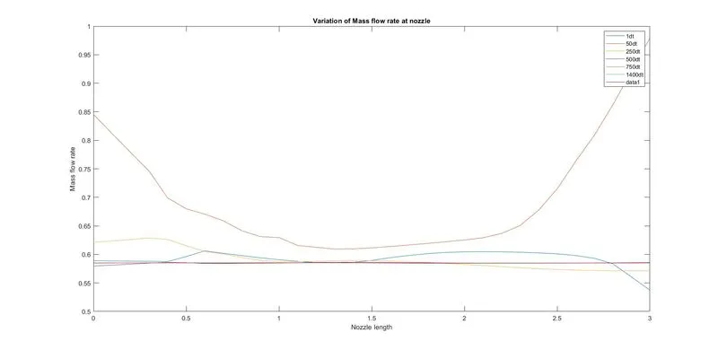
Mass flow rate at different time steps
Code for Conservative form:
clc
close all
clear all
%inputs
n=31;
x=linspace(0,3,n);
dx=x(2)-x(1);
gamma=1.4;
for i=1:n
if x(i) <= 0.5
rho(i)=1;
t(i)=1;
end
if x(i) > 0.5 && x(i) <= 1.5
rho(i)=1-0.366*(x(i)-0.5);
t(i)=1-0.167*(x(i)-0.5);
end
if x(i) > 1.5 && x(i) <= 3.5
rho(i)=0.634-0.3879*(x(i)-1.5);
t(i)=0.833-0.3507*(x(i)-1.5);
end
end
%time step
nt=1400;
%dt=min(0.5*dx./(sqrt(t)+v));
dt=0.02;
th=round(n/2);
%calculate intital profile
% rho=1-0.3146*x;
% t= 1-0.2314*x;
% v=(0.1+1.09*x).*t.^0.5;
%area
a=1+2.2*(x-1.5).^2;
v=0.59./(rho.*a);
U1=rho.*a;
U2=U1.*v;
U3=U1.*(t/(gamma-1)+(gamma/2)*v.^2);
F1=U2;
F2=U2.^2./U1 + gamma/(gamma-1)*(U3-(gamma/2)*(U2.^2/U1));
F3=gamma*U2.*U3./U1 - 0.5* gamma*(gamma-1)*(U2.^3/U1.^2);
cfl=max((v+sqrt(t))*dt/dx);
%outer time loop
for k=1:nt
%predictor method
U1_old=U1;
U2_old=U2;
U3_old=U3;
F1=U2;
F2=U2.^2./U1 + (gamma-1)/(gamma)*(U3-(gamma/2)*(U2.^2./U1));
F3=gamma*U2.*U3./U1 - 0.5* gamma*(gamma-1)*(U2.^3./U1.^2);
for j=2:n-1
%continuity equation
dU1dt_p(j)=-(F1(j+1)-F1(j))/dx;
%momentum equation
J2=(1/gamma)*rho(j)*t(j)*(a(j+1)-a(j))/dx;
dU2dt_p(j)= -(F2(j+1)-F2(j))/dx + J2;
%energy equation
dU3dt_p(j)=-(F3(j+1)-F3(j))/dx;
%solution update
U1(j)=U1(j)+dU1dt_p(j)*dt;
U2(j)=U2(j)+dU2dt_p(j)*dt;
U3(j)=U3(j)+dU3dt_p(j)*dt;
end
% Predictor update
rho= U1./a;
t=(gamma-1)*(U3./U1 - (gamma/2)*(U2./U1).^2)
F1=U2;
F2=U2.^2./U1 + (gamma-1)/(gamma)*(U3-(gamma/2)*(U2.^2./U1));
F3=gamma*U2.*U3./U1 - 0.5* gamma*(gamma-1)*(U2.^3./U1.^2);
%corrrector method
for j=2:n-1
%continuity equation
dU1dt_c(j)=-(F1(j)-F1(j-1))/dx;
%momentum equation
J2=(1/gamma)*rho(j)*t(j)*(a(j)-a(j-1))/dx;
dU2dt_c(j)= -(F2(j)-F2(j-1))/dx + J2;
%energy equation
dU3dt_c(j)=-(F3(j)-F3(j-1))/dx;
end
%compute average time derivative
dU1dt=0.5*(dU1dt_p+dU1dt_c);
dU2dt=0.5*(dU2dt_p+dU2dt_c);
dU3dt=0.5*(dU3dt_p+dU3dt_c);
for i=2:n-1
%solution update
U1(i)=U1_old(i)+dU1dt(i)*dt;
U2(i)=U2_old(i)+dU2dt(i)*dt;
U3(i)=U3_old(i)+dU3dt(i)*dt;
end
%BC
%inlet
U1(1)=rho(1)*a(1);
U2(1)=2*U2(2)-U2(3);
U3(1)=U1(1)*(t(1)/(gamma-1)+0.5*gamma*v(1)^2);
%outlet
U1(n)=2*U1(n-1)-U1(n-2);
U2(n)=2*U2(n-1)-U2(n-2);
U3(n)=2*U3(n-1)-U3(n-2);
% Predictor update
rho= U1./a;
t=(gamma-1)*(U3./U1 - (gamma/2)*(U2./U1).^2);
v=U2./U1;
p=rho.*t; %pressure
M=v./sqrt(t); %Mach number
m=rho.*a.*v; %mass flow rate
hold on
if k==1
figure(3)
plot(x,m);
hold on
end
if k==50
figure(3)
plot(x,m);
hold on
end
if k==250
figure(3)
plot(x,m);
hold on
end
if k==500
figure(3)
plot(x,m);
hold on
end
if k==750
figure(3)
plot(x,m);
hold on
end
if k==1400
figure(3)
plot(x,m);
hold on
xlabel('Nozzle length')
ylabel('Mass flow rate')
title("Variation of Mass flow rate at nozzle for different time steps")
legend('1dt','50dt','250dt','500dt','750dt','1400dt')
end
rho_throat(k)=rho(th);
v_throat(k)=v(th);
t_throat(k)=t(th);
p_throat(k)=p(th);
M_throat(k)=M(th);
end
% pause(0.003)
figure(1)
subplot(5,1,1)
plot(x,v)
xlabel('Nozzle length')
ylabel('Velocity')
title("Variation of velocity at nozzle")
subplot(5,1,2)
plot(x,rho)
xlabel('Nozzle length')
ylabel('Density')
title("Variation of density at nozzle")
subplot(5,1,3)
plot(x,t)
xlabel('Nozzle length')
ylabel('Temperature')
title("Variation of temperature at nozzle")
subplot(5,1,4)
plot(x,p)
xlabel('Nozzle length')
ylabel('Pressure')
title("Variation of pressure at nozzle")
subplot(5,1,5)
plot(x,M)
xlabel('Nozzle length')
ylabel('Mach Number')
title("Variation of Mach Number at nozzle")
figure(2)
subplot(5,1,1)
plot(v_throat)
xlabel('Time step')
ylabel('Velocity')
title("Transient Variation of primitive variable at throat")
subplot(5,1,2)
plot(rho_throat)
xlabel('Time step')
ylabel('Density')
% title("Variation of density at nozzle")
subplot(5,1,3)
plot(t_throat)
xlabel('Time step')
ylabel('Temperature')
% title("Variation of temperature at nozzle")
subplot(5,1,4)
plot(p_throat)
xlabel('Time step')
ylabel('Pressure')
% title("Variation of pressure at nozzle")
subplot(5,1,5)
plot(M_throat)
xlabel('Time step')
ylabel('Mach Number')
% title("Variation of Mach Number at nozzle")
figure(3)
plot(x,m)
xlabel('Nozzle length')
ylabel('Mass flow rate')
title("Variation of Mass flow rate at nozzle")
Flow parameters at nozzle
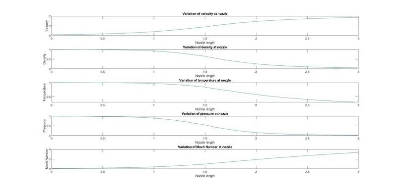
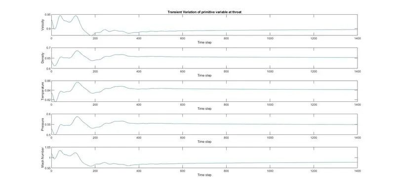
Transient variation of primitive variable at throat
Mass flow rate at different time steps
Grid independence study:
I have increased the grid size to higher value (60) and the plots were look stable as well as similar to existing grid size(31).
But if I increased the grid size to about 90 there were some changes in mass flow rate plot.
Conclusion:
The plots from both the conservative and non-conservative form were look similar but there were more oscillations in non-conservative form than conservative form. We can conclude that conservative form provides stable solution earlier than nonconservative form.