Week 7 - Simulation of a 1D Super-sonic nozzle flow simulation using Macormack Method
Aim:
To simulate the isentropic flow through a quasi 1D subsonic-supersonic nozzle and to derive both the conservation and non-conservation forms of the governing equations and sovle them using the MacCormack's technique.
Supporting equations:
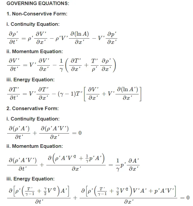
Technique employed: Maccormack method
Matlab code:
clear all
close all
clc
l=3;
% time steps
nt=1400;
cfl=0.5;

% ratio of specific heats
g=1.4;
gridsize=input(' enter your option for grid size(1 for n=31,2 for n=61)=')
if gridsize==1
    n=31;
    x=linspace(0,l,n);
    dx=x(2)-x(1);
    a=1+2.2*(x-1.5).^2;
    [rho_c,mach_c,t_c,v_c,m_c,p_c]=conservation(n,l,dx,g,nt,a,x);
    [rho_nc,t_nc,v_nc,m_nc,p_nc]=nonconservation(n,l,dx,g,a,nt,x,cfl);
    figure(1)
    plot(x,m_c,'r')
    hold on
    plot(x,m_nc,'g')
    xlabel('non dimentional distance')
    ylabel('mass flow rate')
    legend('conservation','nonconservation')
    title('variation of normalised mass flow rate')
    hold off

    figure(2)
    subplot(4,1,1)
    plot(x,rho_c,'b')
    hold on
    plot(x,rho_nc,'.','color','bla','markersize',10)
    xlabel('non dimentional distance')
    ylabel('density')
    legend('conservation','nonconservation')
    title('primitive variables')

    subplot(4,1,2)
    plot(x,p_c,'r')
    hold on
    plot(x,p_nc,'.','color','bla','markersize',10)
    xlabel('non dimentional distance')
    ylabel('pressure')
    legend('conservation','nonconservation')

    subplot(4,1,3)
    plot(x,t_c,'y')
    hold on
    plot(x,t_nc,'.','color','bla','markersize',10)
    xlabel('non dimentional distance')
    ylabel('temperature')
    legend('conservation','nonconservation')

    subplot(4,1,4)
    plot(x,v_c,'m')
    hold on
    plot(x,v_nc,'.','color','bla','markersize',10)
    xlabel('non dimentional distance')
    ylabel('velocity')
    legend('conservation','nonconservation')

end

if gridsize==2
    n=61;
    x=linspace(0,l,n);
    dx=x(2)-x(1);
    a=1+2.2*(x-1.5).^2;
    [rho_c,mach_c,t_c,v_c,m_c,p_c]=conservation(n,l,dx,g,nt,a,x);
    [rho_nc,t_nc,v_nc,m_nc,p_nc]=nonconservation(n,l,dx,g,a,nt,x,dt);
    figure(1)
    plot(x,m_c,'r')
    hold on
    plot(x,m_nc,'g')
    xlabel('non dimentional distance')
    ylabel('mass flow rate')
    legend('conservation','nonconservation')
    title('variation of normalised mass flow rate')
    hold off

    figure(2)
    subplot(4,1,1)
    plot(x,rho_c,'b')
    hold on
    plot(x,rho_nc,'.','color','g','markersize',10)
    xlabel('non dimentional distance')
    ylabel('density')
    legend('conservation','nonconservation')
    title('primitive variables')

    subplot(4,1,2)
    plot(x,p_c,'r')
    hold on
    plot(x,p_nc,'.','color','bla','markersize',10)
    xlabel('non dimentional distance')
    ylabel('pressure')
    legend('conservation','nonconservation')

    subplot(4,1,3)
    plot(x,t_c,'y')
    hold on
    plot(x,t_nc,'.','color','bla','markersize',10)
    xlabel('non dimentional distance')
    ylabel('temperature')
    legend('conservation','nonconservation')

    subplot(4,1,4)
    plot(x,v_c,'m')
    hold on
    plot(x,v_nc,'.','color','bla','markersize',10)
    xlabel('non dimentional distance')
    ylabel('velocity')
    legend('conservation','nonconservation')
end
sub functions:
function [rho_c,mach_c,t_c,v_c,m_c,p_c]=conservation(n,l,dx,g,nt,a,x)

for i=1:n
    if x(i)<=0.5
        rho_c(i)=1;
        t_c(i)=1;
    elseif (x(i)>0.5)&&(x(i)<=1.5)
        rho_c(i)=1-0.366*(x(i)-0.5);
        t_c(i)=1-0.167*(x(i)-0.5);
    elseif (x(i)>=0.5)&&(x(i)<=3)
        rho_c(i)=0.634-0.3879*(x(i)-1.5);
        t_c(i)=0.833-0.3507*(x(i)-1.5);
    end
end
v_c=0.59./(rho_c.*a);
mach_c=v_c./(t_c.^(0.5));
m_c=rho_c.*a.*v_c;
p_c=rho_c.*t_c;
cfl=.5;
u1=rho_c.*a;
u2=rho_c.*a.*v_c;
u3=rho_c.*a.*(t_c./(g-1)+(0.5*g*(v_c.^2)));
dt=min(cfl*(dx./(t_c.^0.5+v_c)));


% initialising flux functions

for k=1:nt
    u1_old=u1;
    u2_old=u2;
    u3_old=u3;

    f1=u2;
    f2=((u2.^2)./u1)+((g-1)/g)*(u3-0.5*g*((u2.^2)./u1));
    f3=(g*(u2.*u3)./u1)-g*(g-1)*0.5*((u2.^3)./(u1.^2));
    for j=2:n-1
        dlogadx=(log(a(j+1))-log(a(j)))/dx;
        %         j2=((g-1)/g)*(u3-0.5*g*((u2.^2)./u1))*dlogadx;
        j2=rho_c(j)*t_c(j)*(1/g)*((a(j+1)-a(j))/dx);

        df1dx=(f1(j+1)-f1(j))/dx;
        df2dx=(f2(j+1)-f2(j))/dx;
        df3dx=(f3(j+1)-f3(j))/dx;
        %         predictor step
        du1dt_p(j)=-df1dx;
        du2dt_p(j)=-df2dx+j2;
        du3dt_p(j)=-df3dx;
        % update
        u1(j)=u1(j)+du1dt_p(j)*dt;
        u2(j)=u2(j)+du2dt_p(j)*dt;
        u3(j)=u3(j)+du3dt_p(j)*dt;
    end
    %update after predictor step
    rho_c=u1./a;
    v_c=u2./u1;
    t_c=(g-1)*((u3./u1)-0.5*g*(v_c.^2));
    p_c=rho_c.*t_c;
    f1=u2;
    f2=((u2.^2)./u1)+((g-1)/g)*(u3-0.5*g*((u2.^2)./u1));
    f3=(g*(u2.*u3)./u1)-g*(g-1)*0.5*((u2.^3)./(u1.^2));
    %     corrector step
    for j=2:n-1
        %         dlogadx_bd=(log(a(j))-log(a(j-1)))/dx;
        %         j2=((g-1)/g)*(u3-0.5*g*((u2.^2)./u1))*dlogadx_bd;
        j2=rho_c(j)*t_c(j)*(1/g)*((a(j)-a(j-1))/dx);
        df1dx=(f1(j)-f1(j-1))/dx;
        df2dx=(f2(j)-f2(j-1))/dx;
        df3dx=(f3(j)-f3(j-1))/dx;
        %         predictor step
        du1dt_c(j)=-df1dx;
        du2dt_c(j)=-df2dx+j2;
        du3dt_c(j)=-df3dx;
    end
    % calculating average
    du1dt=0.5*(du1dt_p+du1dt_c);
    du2dt=0.5*(du2dt_p+du2dt_c);
    du3dt=0.5*(du3dt_p+du3dt_c);
    for b=2:n-1
        u1(b)=u1_old(b)+du1dt(b)*dt;
        u2(b)=u2_old(b)+du2dt(b)*dt;
        u3(b)=u3_old(b)+du3dt(b)*dt;
    end
    %      conditions
    % initial
    u1(1)=rho_c(1)*a(1);
    u2(1)=2*u2(2)-u2(3);
    v_c(1)=u2(1)/u1(1);
    u3(1)=u1(1)*((t_c(1)/(g-1))+((g*0.5)*v_c(1)^2));
    % boundary
    u1(n)=2*u1(n-1)-u1(n-2);
    u2(n)=2*u2(n-1)-u2(n-2);
    u3(n)=2*u3(n-1)-u3(n-2);

    %     primitive variables
    rho_c=u1./a;
    v_c=u2./u1;
    t_c=(g-1)*((u3./u1)-0.5*g*v_c.^2);
    p_c=rho_c.*t_c;
    mach_c=v_c./(t_c.^0.5);
    m_c=rho_c.*a.*v_c;
    figure(3)
    if k==50
        plot(x,m_c,'b')
        hold on
    elseif k==100
        plot(x,m_c,'r')
    elseif k==150
        plot(x,m_c,'g')
        xlabel('non dimentional distance')
        ylabel('mass flow rate(conservation)')
        legend('50\deltat','100\deltat','150\deltat')
        title('variation of mass flow rate(conservation) with time steps')
    end
end


function [rho_nc,t_nc,v_nc,m_nc,p_nc]=nonconservation(n,l,dx,g,a,nt,x,cfl)
rho_nc=1-0.3146*x;
t_nc=1-0.2314*x;  %t is temp
v_nc=(0.1+1.09*x).*t_nc.^0.5;
g=1.4;
dt=min(cfl*(dx./(t_nc.^0.5+v_nc)));
% formulas
for k=1:nt
    rho_oldnc=rho_nc;
    t_oldnc=t_nc;
    v_oldnc=v_nc;
    for j=2:n-1
        dvdx=(v_nc(j+1)-v_nc(j))/dx;
        dlogadx=(log(a(j+1))-log(a(j)))/dx;
        drhodx=(rho_nc(j+1)-rho_nc(j))/dx;
        dtdx=(t_nc(j+1)-t_nc(j))/dx;

        drhodt_p(j)=-rho_nc(j)*dvdx-rho_nc(j)*v_nc(j)*dlogadx-v_nc(j)*drhodx;
        dvdt_p(j)=-v_nc(j)*dvdx-(1/g)*(dtdx+(t_nc(j)/rho_nc(j))*drhodx);
        dtdt_p(j)=-v_nc(j)*dtdx-(g-1)*t_nc(j)*(dvdx+v_nc(j)* dlogadx);

        %        update
        v_nc(j)=v_nc(j)+dvdt_p(j)*dt;
        rho_nc(j)=rho_nc(j)+drhodt_p(j)*dt;
        t_nc(j)=t_nc(j)+dtdt_p(j)*dt;
    end
    for j=2:n-1
        dvdx=(v_nc(j)-v_nc(j-1))/dx;
        dlogadx=(log(a(j))-log(a(j-1)))/dx;
        drhodx=(rho_nc(j)-rho_nc(j-1))/dx;
        dtdx=(t_nc(j)-t_nc(j-1))/dx;

        drhodt_c(j)=-rho_nc(j)*dvdx-rho_nc(j)*v_nc(j)*dlogadx-v_nc(j)*drhodx;
        dvdt_c(j)=-v_nc(j)*dvdx-(1/g)*(dtdx+(t_nc(j)/rho_nc(j))*drhodx);
        dtdt_c(j)=-v_nc(j)*dtdx-(g-1)*t_nc(j)*(dvdx+v_nc(j)* dlogadx);

    end
    %        avg
    drhodt=0.5*(drhodt_c+drhodt_p);
    dvdt=0.5*(dvdt_c+dvdt_p);
    dtdt=0.5*(dtdt_c+dtdt_p);
    for l=2:n-1
        v_nc(l)=v_oldnc(l)+dvdt(l)*dt;
        rho_nc(l)=rho_oldnc(l)+drhodt(l)*dt;
        t_nc(l)=t_oldnc(l)+dtdt(l)*dt;
    end
    %     apply boundary conditions
    v_nc(1)=2*v_nc(2)-v_nc(3);
    rho_nc(1)=1;
    t_nc(1)=1;
    v_nc(n)=2*v_nc(n-1)-v_nc(n-2);
    rho_nc(n)=2*rho_nc(n-1)-rho_nc(n-2);
    t_nc(n)=2*t_nc(n-1)-t_nc(n-2);
    mach_nc=v_nc./(t_nc.^(0.5));
    m_nc=rho_nc.*a.*v_nc;
    p_nc=rho_nc.*t_nc;

    figure(4)
    if k==50
        plot(x,m_nc,'b')
        hold on
    elseif k==100
        plot(x,m_nc,'r')
    elseif k==150
        plot(x,m_nc,'g')
        xlabel('non dimentional distance')
        ylabel('mass flow rate(nonconservation)')
        legend('50\deltat','100\deltat','150\deltat')
        title('variation of mass flow rate(nonconservation) with time steps')
    end
end
Results and discussions:
As we see from the results that if we change the grid size there is no change in the graphs obtained. thus the system is grid independent.
Normalised mass flow rate in case of conserved flow remains unchanged throughout or changes slightly. this is not the case with nonconservation as there is an abrubt change in mass flow rate. this is attributed to the fact that in conservation method, mass flow rate is kept constant by deriving equations using fixed control volume. in the latter mass flow rate changes to account for the density change to maintain the shape of the movable control volume constant.
initially when the time steps were less, mass flow rate in both conservation and non conservation form suffers changes. but as the time step increases mass flow rate in conservation method reaches a steady state value.
as the nozzle is convergent divergent nozzle the primitive variables like non dimentional pressure,non dimentional temperature ,non dimentional density decreases as we move from one end of the nozzle to other. but the non dimentional velocity increases as we move from one end of the nozzle to other. this is because the flow velocity increases throughout the flow.