Week 7 - Simulation of a 1D Super-sonic nozzle flow simulation using Macormack Method

Objective: In this challenge, we will simulate isentropic flow through a quasi 1D subsonic-supersonic nozzle using MacCormack's method by deriving and then solving both the conservation and non-conservation forms of the governing equations.

The Objective of this challenge is as follows:

• Steady-state distribution of primitive variables inside the nozzle.
• Time-wise variation of the primitive variables.
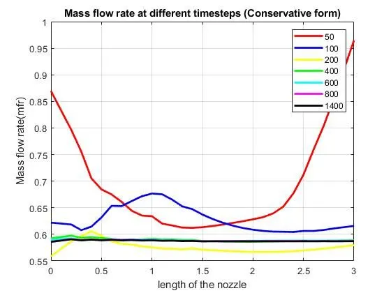
• Variation of Mass flow rate distribution inside the nozzle at different time steps during the time-marching process.
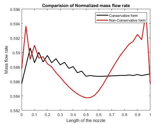
• Comparison of Normalized mass flow rate distributions of both forms.
• grid independence test on the solution.

Description:

The converging-diverging nozzle is attached to a reservoir where velocity Vo is minimum at the inlet as the flow is subsonic and at exit is supersonic. The pressure and temperature are denoted by Po and To and at the throat of the nozzle, the Mach number is 1.

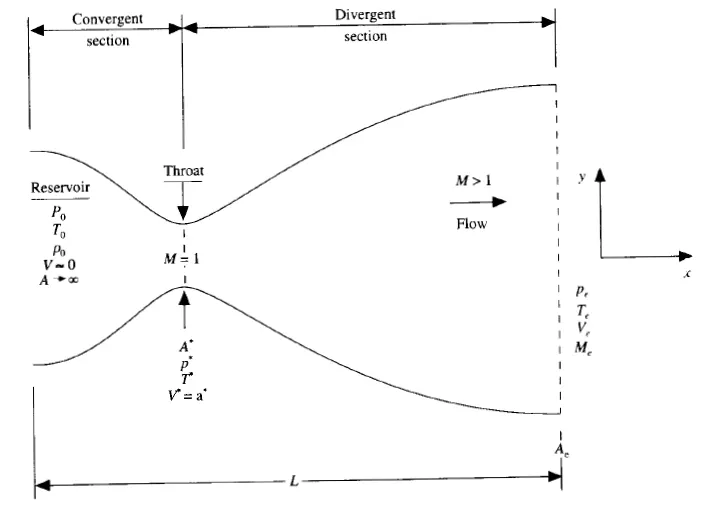
In this solution, governing equations that are in conservative form and non-conservative form are solved using MacCormack's method for discretization.

MacCormack's method:

MacCormack's technique is a variant of the Lax-Wendroff approach but is much simpler in its application. This method is an explicit finite difference technique that is second-order accurate in both time and space. This method gives better results for the hyperbolic equation and can provide stable solutions in the presence of shock. Thus, they are used in nozzle flow problems. In the MacCormack method, a combination of both forward and backward differencing schemes are used to solve the primitive variables.

This method solves in two steps where `Delta t` is used as time step are as follows:

• Predictor step: In this step, The spatial derivatives in the 1st order equation is replaced by using a forward difference scheme.
• Corrector step: The spatial derivatives in the 1st order equation is replaced by using a backward difference scheme.

After using the steps and updating the solution, the average time derivative is determined and the final solution is updated.

Governing equations for Non-conservative form:

Governing equations for Conservative form:

These equations are used to analyse the problem by giving analytical solutions with different numerical outputs.

Main Program for solving 1D supersonic nozzle:

clear all
close all
clc


% inputs
n = 31;
x = linspace(0,3,n);
dx = x(2) - x(1);
gamma = 1.4;
nt = 1400;    % time steps

a = 1 + 2.2*(x-1.5).^2;  % area

% Non Conservative form
tic
[rho_NC,v_NC,t_NC,mfr_NC,Mac_NC,p_NC,rho_tNC,t_tNC,mfr_tNC,Mac_tNC,p_tNC] = NC_fun(x,dx,n,a,gamma,nt);
time_NC = toc

%Conservative form
tic
[rho_C,v_C,t_C,p_C,Mac_C,mfr_C,rho_tC,v_tC,t_tC,p_tC,Mac_tC,mfr_tC] = C_fun(x,n,dx,gamma,a,nt)
time_C = toc

%plotting for Steady state distribution of primitive variables
figure(3)
%Density
subplot(4,1,1)
plot(x,rho_C,'k','linewidth',1.5)
hold on
plot(x,rho_NC,'*','linewidth',1.5)
hold on
grid on
title('Steady state distribution of primitive variables inside the nozzle')
xlabel('Length of the Nozzle')
ylabel('Density')
legend('Conservative form','Non Conservative form')
%Pressure
subplot(4,1,2)
plot(x,p_C,'k','linewidth',1.5)
hold on
plot(x,p_NC,'*','linewidth',1.5)
hold on
grid on
xlabel('Length of the Nozzle')
ylabel('Pressure')
%Temperature
subplot(4,1,3)
plot(x,t_C,'k','linewidth',1.5)
hold on
plot(x,t_NC,'*','linewidth',1.5)
hold on
grid on
xlabel('Length of the Nozzle')
ylabel('Temperature')
%Mach number
subplot(4,1,4)
plot(x,Mac_C,'k','linewidth',1.5)
hold on
plot(x,Mac_NC,'*','linewidth',1.5)
hold on
xlabel('Length of the Nozzle')
ylabel('Mach number')
grid on
hold on

%Plot for time-wise variation of primitive variable at throat
figure(4)
%Density
subplot(4,1,1)
plot(1:nt,rho_tC,'k','linewidth',2)
hold on
plot(1:nt,rho_tNC,'r','linewidth',2)
hold on
grid on
title('Time-wise distribution of primitive variable at throat')
xlabel('Length of the Nozzle')
ylabel('Density')
legend('Conservative form','Non Conservative form')
%Pressure
subplot(4,1,2)
plot(1:nt,p_tC,'k','linewidth',2)
hold on
plot(1:nt,p_tNC,'r','linewidth',2)
hold on
grid on
xlabel('Length of the Nozzle')
ylabel('Pressure')
%Temperature
subplot(4,1,3)
plot(1:nt,t_tC,'k','linewidth',2)
hold on
plot(1:nt,t_tNC,'r','linewidth',2)
hold on
grid on
xlabel('Length of the Nozzle')
ylabel('Temperature')
%Mach number
subplot(4,1,4)
plot(1:nt,Mac_tC,'k','linewidth',2)
hold on
plot(1:nt,Mac_tNC,'r','linewidth',2)
hold on
xlabel('Length of the Nozzle')
ylabel('Mach number')
grid on
hold on

%plot for comparision of Normalized mass flow rate distributions
figure(5)
plot(x/3,mfr_C,'k','linewidth',2)
hold on
plot(x/3,mfr_NC,'r','linewidth',2)
title('Comparision of Normalized mass flow rate')
legend('Conservative form','Non-Conservative form')
xlabel('Length of the nozzle')
ylabel('Mass flow rate')

Function for Non-conservative form:

%Function for Non Conservative form
function [rho_NC,v_NC,t_NC,mfr_NC,Mac_NC,p_NC,rho_tNC,t_tNC,mfr_tNC,Mac_tNC,p_tNC] = NC_fun(x,dx,n,a,gamma,nt)


thr = find(a==1);                  %Throat

% calcuate intial profiles
rho_NC = 1-0.3146*x;               %Density
t_NC = 1-0.2314*x;                 %Temperature
v_NC = (0.1 + 1.09*x).*t_NC.^0.5;  %velocity

mfr_NC = rho_NC.*a.*v_NC;          %Mass flow rate
p_NC = rho_NC.*t_NC;               %pressure

c = 0.5;                           %Courant number
dt = min(c*(dx./((t_NC.^0.5) + v_NC)));

% outer time loop
for k = 1:nt
    
    rho_old_NC = rho_NC;
    v_old_NC = v_NC;
    t_old_NC = t_NC;
    
    %Preditor method
    for j = 2:n-1        
        dvdx = (v_NC(j+1) - v_NC(j))/dx;
        drhodx = (rho_NC(j+1) - rho_NC(j))/dx;
        dtdx = (t_NC(j+1) - t_NC(j))/dx;
        dlogadx = (log(a(j+1)) - log(a(j)))/dx;
        
        %Continuty equation
        drhodt_p(j) = -rho_NC(j)*dvdx - rho_NC(j)*v_NC(j)*dlogadx - v_NC(j)*drhodx;
        
        %Momenturn equation 
        dvdt_p(j) = -v_NC(j)*dvdx - (1/gamma)*(dtdx + (t_NC(j)/rho_NC(j))*drhodx);
        
        %Energy equation
        dtdt_p(j) = -v_NC(j)*dtdx - (gamma-1)*t_NC(j)*(dvdx + v_NC(j)*dlogadx);
   
    %Solution update 
    rho_NC(j) = rho_NC(j) + drhodt_p(j)*dt;
    v_NC(j) = v_NC(j) + dvdt_p(j)*dt;
    t_NC(j) = t_NC(j) + dtdt_p(j)*dt;
    
    end
    
    
    %Corrector method
    for j = 2:n-1        
        dvdx = (v_NC(j) - v_NC(j-1))/dx;
        drhodx = (rho_NC(j) - rho_NC(j-1))/dx;
        dtdx = (t_NC(j) - t_NC(j-1))/dx;
        dlogadx = (log(a(j)) - log(a(j-1)))/dx;
        
        %Continuty equation
        drhodt_c(j) = -rho_NC(j)*dvdx - rho_NC(j)*v_NC(j)*dlogadx - v_NC(j)*drhodx;
        
        %Momenturn equation 
        dvdt_c(j) = -v_NC(j)*dvdx - (1/gamma)*(dtdx + (t_NC(j)/rho_NC(j))*drhodx);
        
        %Energy equation
        dtdt_c(j) = -v_NC(j)*dtdx - (gamma-1)*t_NC(j)*(dvdx + v_NC(j)*dlogadx);
    end
    
    %Compute the average time derivative
    
    drhodt = 0.5*(drhodt_p + drhodt_c);
    dvdt = 0.5*(dvdt_p + dvdt_c);
    dtdt = 0.5*(dtdt_p + dtdt_c);
    
    %Final solution update
    
    for i = 2:n-1
        rho_NC(i) = rho_old_NC(i) + drhodt(i)*dt;
        v_NC(i) = v_old_NC(i) + dvdt(i)*dt;
        t_NC(i) = t_old_NC(i) + dtdt(i)*dt;
    end
    
    %Apply boundary conditions
    %inlet
    v_NC(1) = 2*v_NC(2) - v_NC(3);
    
    %outlet
    rho_NC(n) = 2*rho_NC(n-1) - rho_NC(n-2);
    v_NC(n) = 2*v_NC(n-1) - v_NC(n-2);
    t_NC(n) = 2*t_NC(n-1) - t_NC(n-2);
    
    
    mfr_NC = rho_NC.*a.*v_NC;
    Mac_NC = v_NC./(t_NC.^0.5);
    p_NC = rho_NC.*t_NC;
   
    %Throat values
    t_tNC(k) = t_NC(thr);
    rho_tNC(k) = rho_NC(thr);
    Mac_tNC(k) = Mac_NC(thr);
    p_tNC(k) = p_NC(thr);
    mfr_tNC(k) = mfr_NC(thr);
    
    %Plotting Mass flow rate inside the nozzle at different time step
    figure(1)
    if k == 50
        plot(x,mfr_NC,'r','linewidth',2)
        hold on
    elseif k == 100
        plot(x,mfr_NC,'b','linewidth',2)
        hold on
    elseif k == 200
        plot(x,mfr_NC,'y','linewidth',2)
        hold on
    elseif k == 400
        plot(x,mfr_NC,'g','linewidth',2)
        hold on
    elseif k == 600
        plot(x,mfr_NC,'c','linewidth',2)
        hold on
    elseif k == 800
        plot(x,mfr_NC,'m','linewidth',2)
    elseif k == 1400
        plot(x,mfr_NC,'k','linewidth',2)
        hold on
        grid on
        title('Mass flow rate at different timesteps (Non-Conservative form)')
        legend('50','100','200','400','600','800','1400')    
        xlabel('length of the nozzle')
        ylabel('Mass flow rate(mfr)')
   end
    
 
    
end   
end

Function for Conservative form:

%Function for Conservative form

function[rho_C,v_C,t_C,p_C,Mac_C,mfr_C,rho_tC,v_tC,t_tC,p_tC,Mac_tC,mfr_tC] = C_fun(x,n,dx,gamma,a,nt)

%Initial conditions
for z=1:length(x)
    if x(z)>=0 && x(z)<0.5
        rho_C(z) = 1;
        t_C(z) = 1;
    elseif x(z)>=0.5 && x(z)<1.5
        rho_C(z) = 1 - (0.366*(x(z) - 0.5));
        t_C(z) = 1 - (0.167*(x(z) - 0.5));
    elseif x(z)>=1.5 && x(z)<=3
        rho_C(z) = 0.634 - (0.3879*(x(z) - 1.5));
        t_C(z) = 0.833 - (0.3507*(x(z) - 1.5));
    end
end


c = 0.5;
thr = find(a==1);

%initial profiles
p_C = rho_C.*t_C;
v_C = 0.59./(rho_C.*a);
mfr_C = rho_C.*a.*v_C;
Mac_C = v_C./(t_C.^0.5);

dt = min(c*(dx./((t_C.^0.5) + v_C)));

%Solution vectors
u1 = rho_C.*a;
u2 = u1.*v_C;
u3 = ((t_C./(gamma-1)) + (gamma*0.5.*(v_C.^2))).*u1;

%Outer timeloop
for k=1:nt    
    %Storing initial values
    u1_old = u1; 
    u2_old = u2; 
    u3_old = u3;
    
    for j = 2:n-1
        %Flux vector
        F1 = u2;
        F2 = ((u2.^2)./u1) + (((gamma - 1)/gamma)*(u3 - (u2.^2./u1*0.5*gamma)));
        F3 = ((gamma.*u2.*u3)./u1) - ((0.5*gamma*(gamma-1)).*((u2.^3)./(u1.^2)));
           
        dlogadx(j) = (log(a(j+1)) - log(a(j)))/dx;
        %Source term
        J2_p(j) = (((gamma-1)/gamma)*(u3(j) - (((u2(j)^2)/u1(j))*0.5*gamma)))*dlogadx(j);
        %Predictor step
        
        %continuity equation
        du1_dt_p(j) = -(F1(j+1) - F1(j))/dx;
        
        %momentum equation
        du2_dt_p(j) = -(F2(j+1) - F2(j))/dx + J2_p(j);
        
        %energy equation
        du3_dt_p(j) = -(F3(j+1) - F3(j))/dx;
        
        %Solution update
        u1(j) = u1(j) + (du1_dt_p(j)*dt);
        u2(j) = u2(j) + (du2_dt_p(j)*dt);
        u3(j) = u3(j) + (du3_dt_p(j)*dt);
    end
    
    %Updating primitives
    v_C = u2./u1;
    t_C = (gamma-1)*((u3./u1) - (gamma*0.5.*v_C.^2));
    rho_C = u1./a;
    
    %Updating Flux vectors
    F1 = u2;
    F2 = ((u2.^2)./u1) + (((gamma-1)/gamma)*(u3-(((u2.^2)./u1)*0.5*gamma)));
    F3 = ((gamma.*u2.*u3)./u1) - ((0.5*gamma*(gamma-1)).*((u2.^3)./(u1.^2)));
    
    %Corrector step
    for j = 2:n-1                 
        dlogadx(j) = (log(a(j)) - log(a(j-1)))/dx;
        %Source term
        J2_c(j) = (((gamma-1)/gamma)*(u3(j) - (((u2(j)^2)/u1(j))*0.5*gamma)))*dlogadx(j);
        %Predictor step
        
        %continuity equation
        du1_dt_c(j) = -(F1(j) - F1(j-1))/dx;
        
        %momentum equation
        du2_dt_c(j) = -(F2(j) - F2(j-1))/dx + J2_c(j);
        
        %energy equation
        du3_dt_c(j) = -(F3(j) - F3(j-1))/dx;
        
    end
    
    %average time derivative
        du1_dt = 0.5*(du1_dt_p + du1_dt_c);
        du2_dt = 0.5*(du2_dt_p + du2_dt_c);
        du3_dt = 0.5*(du3_dt_p + du3_dt_c);
    
    %Final solution update
    for i = 2:n-1
        u1(i) = u1_old(i) + du1_dt(i)*dt;
        u2(i) = u2_old(i) + du2_dt(i)*dt;
        u3(i) = u3_old(i) + du3_dt(i)*dt;
    end
    
    %inlet boundary condition
    u1(1) = rho_C(1)*a(1);
    u2(1) = 2*u2(2) - u2(3);
    u3(1) = u1(1)*((t_C(1)/(gamma-1)) + (gamma*0.5*(u2(1)/u1(1))^2));
    
    %outlet boundary condition
    u1(n) = 2*u1(n-1) - u1(n-2);
    u2(n) = 2*u2(n-1) - u2(n-2);
    u3(n) = 2*u3(n-1) - u3(n-2);
    
    %Final update
    v_C = u2./u1;
    t_C = (gamma-1).*((u3./u1) - (gamma*0.5.*v_C.^2));
    rho_C = u1./a;
    Mac_C = v_C./(t_C.^0.5);
    p_C = rho_C.*t_C;
    mfr_C = rho_C.*a.*v_C;
    
    %Throat values
    t_tC(k) = t_C(thr);
    rho_tC(k) = rho_C(thr);
    mfr_tC(k) = mfr_C(thr);
    Mac_tC(k) = Mac_C(thr);
    p_tC(k) = p_C(thr);
    v_tC(k) = v_C(thr);
    
    %Plotting Mass flow rate inside the nozzle at different time step
    figure(2)
    if k == 50
        plot(x,mfr_C,'r','linewidth',2)
        hold on
    elseif k == 100
        plot(x,mfr_C,'b','linewidth',2)
        hold on
    elseif k == 200
        plot(x,mfr_C,'y','linewidth',2)
        hold on
    elseif k == 400
        plot(x,mfr_C,'g','linewidth',2)
        hold on
    elseif k == 600
        plot(x,mfr_C,'c','linewidth',2)
        hold on
    elseif k == 800
        plot(x,mfr_C,'m','linewidth',2)
    elseif k == 1400
        plot(x,mfr_C,'k','linewidth',2)
        hold on
        grid on
        title('Mass flow rate at different timesteps (Conservative form)')
        legend('50','100','200','400','600','800','1400')    
        xlabel('length of the nozzle')
        ylabel('Mass flow rate(mfr)')
   end
      
end   
end

Results:

1. Steady-state distribution of primitive variables inside the nozzle:

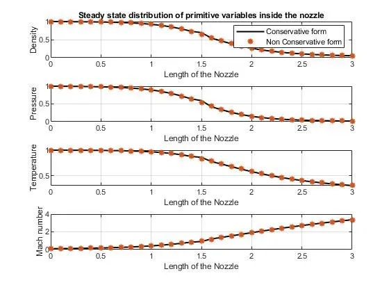
Observation:

Both forms have a similar solution. we could see as the Mac number increases the pressure, density and temperature will drop at the exit of the nozzle. and only the velocity of the flow will be increased.

2. Time-wise distribution of primitive variables:

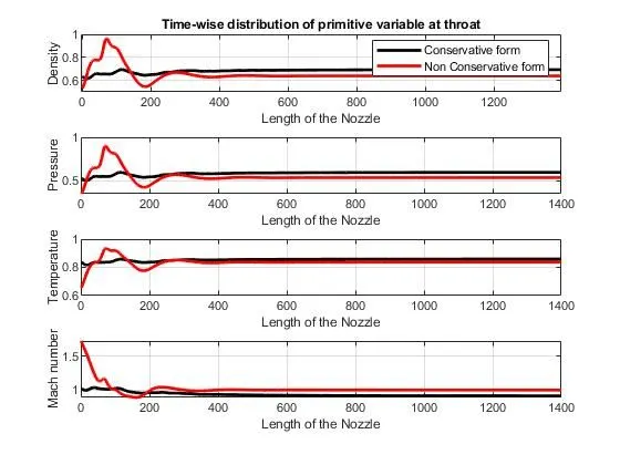
Observation:

As we could see a slight difference in these forms. the Non-conservation form lies closer to the exact values when compared to the conservation form, as the Non-conservation form produces more accurate results for the primitive variables.

3. Variation of Mass flow rate distribution inside the nozzle at different time steps during the time-marching process:

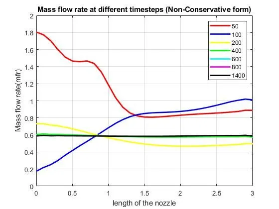
Observation:

From the above plots, We could see both forms getting a steady state after the 400th timestep.

5. Comparison of Normalized mass flow rate distributions of both forms:

Observation:

• The conservative form produces fewer fluctuations compared to the Non-conservative form.
• As in Conservative form, the mass flow is a dependent variable in the equation, unlike the Non-conservative form.
• This produces more accurate results for the flux variables.

6. Grid independence test:

	density ratio `(rhoast)/(rhocirc)`	Temperature ratio `(tast)/(tcirc)`	Pressure ratio `(past)/(pcirc)`	Mach number(M)	Time taken (sec)
Non-conservative form n = 31	0.638	0.836	0.534	0.999	4.4
Conservative form n = 31	0.652	0.841	0.548	0.977	3.4
Non-Conservative form n = 61	0.637	0.835	0.532	0.999	3.6
conservative form n = 61	0.638	0.835	0.533	0.997	4.6
Non-Conservative form n = 91	0.640	0.837	0.536	1.002	3.1
Conservative form n = 91	0.638	0.836	0.533	0.999	6.7
Exact solution	0.639	0.836	0.534	0.99

Observation:

• Here, We have increased the grid points from 31 to 61 and 91 and tabulated them using primitive variables.
• As we can see, the accuracy of the solution increases slightly by increasing the number of grid points.
• the non-conservation form is much closer to the exact solution than the conservation form.
• Calculating variables like flux and source variables takes time in Conservation form and thus time taking for non-conservation form is faster than Conservation form.
• Thus, the non-conservative form has more overall accuracy than the conservation form.
• Finally, we can conclude that the solution is Grid dependent.