Week 7 - Simulation of a 1D Super-sonic nozzle flow simulation using Macormack Method
main program:
clear all
close all
clc

%input variables
n=31; %no. of grid points
x=linspace(0,3,n);
dx=x(2)-x(1);
gamma = 1.4;
nt=1400 % no. of time step
a=1+2.2*(x-1.5).^2;

%exact solution
  rho_exact_n = 0.634*ones(1,1400);
  t_exact_n = 0.833*ones(1,1400);
  p_exact_n = 0.528*ones(1,1400);
  M_exact_n = 1*ones(1,1400);

tic;
[v_n,rho_n,t_n,m_n,M_n,p_n,v_t,rho_t,t_t,m_t,M_t,p_t,v_res_n,rho_res_n,t_res_n] = non_conservative_form(x,n,gamma,nt,dx,a);
non_conservative_execution_time=toc;

%hold on

tic;
[v_c,rho_c,t_c,m_c,M_c,p_c,v_tc,rho_tc,t_tc,m_tc,M_tc,p_tc,v_res_c,rho_res_c,t_res_c] = conservative_form(x,n,gamma,nt,dx,a);
conservative_execution_time=toc;

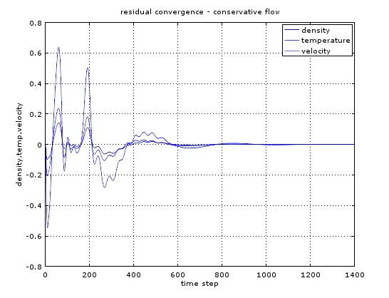
%%conservative flow residual plot
figure(8)
      plot(rho_res_c)
    hold on
     plot(t_res_c)
      hold on
      plot(v_res_c)
xlabel('time step')
ylabel('density,temp,velocity')
title('residual convergence - conservative flow')
legend('density','temperature','velocity')
grid on

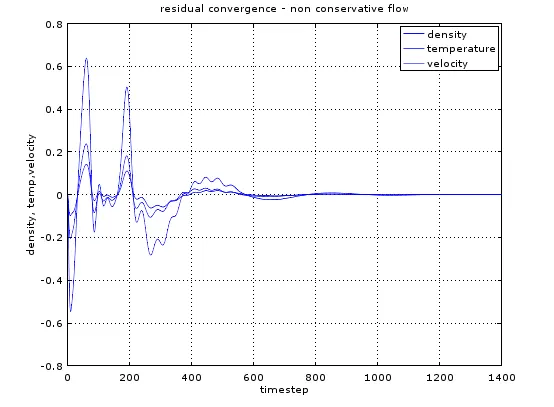
%% non-conservation flow -residual plot
figure(7)
  plot(rho_res_c)
  hold on
plot(t_res_c)
hold on
plot(v_res_c)
xlabel('timestep')
ylabel('density, temp,velocity')
title('residual convergence - non conservative flow')
legend('density','temperature','velocity')
grid on

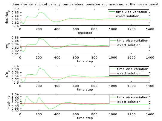
%%conservative form time wise variation of density, pressure,temperature and mach number
figure(6)
subplot(4,1,1)
plot(rho_tc,'g')
hold on
plot(rho_exact_n,'r')
xlabel('timestep')
ylabel('rho/{rho_0}')
title('time wise variation of density, temperature, pressure and mach no. at the nozzle throat')
legend('time wise variation ','exact solution')

subplot(4,1,2)
plot(t_tc,'g')
hold on
plot(t_exact_n,'r')
xlabel('time step')
ylabel('t/{t_0}')
legend('time wise variation','exact solution')


subplot(4,1,3)
plot(p_tc,'g')
hold on
plot(p_exact_n,'r')
xlabel('time step')
ylabel('p/{p_0}')
legend('time wise variation','exact solution')

subplot(4,1,4)
plot(M_tc,'g')
hold on
plot(M_exact_n,'r')
xlabel('time step')
ylabel('mach no')
legend('time wise variation','exact solution')

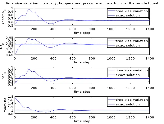
%%non conservative form time wise variation of density, pressure, temperature and mach number
figure(5)
subplot(4,1,1)
plot(rho_t)
hold on
plot(rho_exact_n)
xlabel('time step')
ylabel('rho/{rho_0}')
legend('time wise variation','exact solution')
title('time wise variation of density, temperature, pressure and mach no. at the nozzle throat')

subplot(4,1,2)
plot(t_t)
hold on
plot(t_exact_n)
xlabel('time step')
ylabel('t/{t_0}')
legend('time wise variation','exact solution')

subplot(4,1,3)
plot(p_t)
hold on
plot(p_exact_n)
xlabel('time step')
ylabel('p/{p_0}')
legend('time wise variation','exact solution')

subplot(4,1,4)
plot(M_t)
hold on
plot(M_exact_n)
xlabel('time step');
ylabel('mach no');
legend('time wise variation','exact solution')

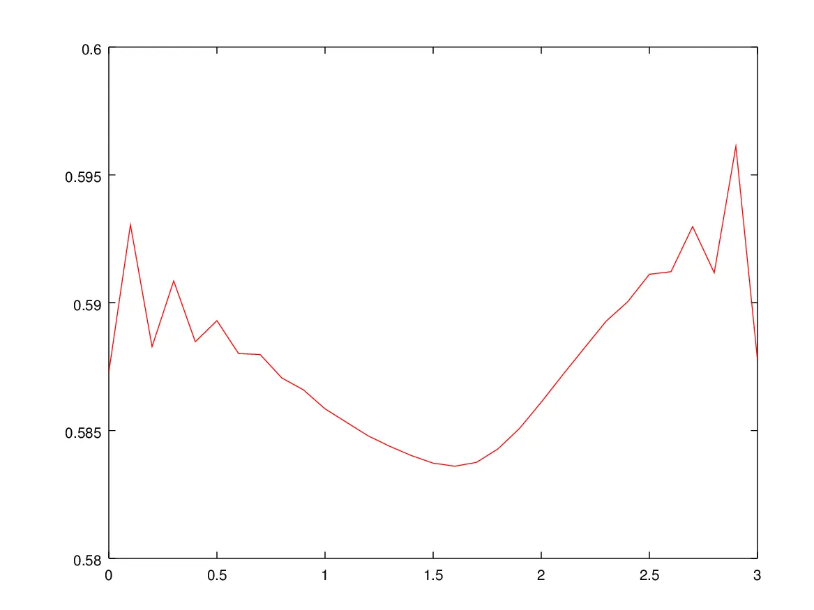
%% non conservative vs conservative form mass flow rate
figure(4)
plot(x,m_n,'r')
hold on
plot(x,m_c,'g')
xlabel('non dimensional mass flow rate')
legend('non conservative flow','conservative flow')
grid on;

%% qualitative aspdects of 1d nozzle flow
figure(3)
subplot(4,1,3)
plot(x,rho_n,'r')
hold on
plot(x,rho_c,'b')
xlabel('length of the nozzle')
ylabel('density')
legend('non-conservative','conservative')
grid on;

subplot(4,1,4)
plot(x,t_n,'r')
hold on
plot(x,t_c,'b')
xlabel('length of the nozzle')
ylabel('temperature')
legend('non-conservative','conservative')
grid on;

subplot(4,1,1)
plot(x,M_n,'r')
hold on
plot(x,M_c,'b')
xlabel('length of the nozzle')
ylabel('mach number')
legend('non-conservative','conservative')
title('qualitative aspects of quasi 1d nozzle flow')
grid on;

subplot(4,1,2)
plot(x,p_n,'r')
hold on
plot(x,p_c,'b')
xlabel('length of the nozzle')
ylabel('pressure')
legend('non-conservative','conservative')
grid on;
non conservative:
function [ v,rho,t,m,M,p,v_th,rho_th,t_th,m_th,M_th,p_th,v_res_n,rho_res_n,t_res_n]=non_conservative_form(x,n,gamma,nt,dx,a)

tic;
% inputs

n=31;
x=linspace(0,3,n);
dx=x(2)-x(1);
gamma=1.4;
th = (n+1)/2;

%calculate initial profiles
rho=1-0.3146*x;
t=1-0.2314*x; % t=temperature
v=(0.1+1.09*x).*t.^0.5;
a=1+2.2*(x-1.5).^2;

%%time steps
nt=1400;
dt=0.01;
%outer time loop,
for k =1:nt
  rho_old=rho;
  v_old=v;
  t_old=t;

  for j=2:n-1

    dvdx=(v(j+1)-v(j))/dx;
    drhodx=(rho(j+1)-rho(j))/dx;
    dtdx=(t(j+1)-t(j))/dx;
    dlogadx=(log(a(j+1))-log(a(j)))/dx;

    %continuity equation
    drhodt_p(j)=-rho(j)*dvdx-rho(j)*v(j)*dlogadx-v(j)*drhodx;
    %momentum equation
    dvdt_p(j)=-v(j)*dvdx-(1/gamma)*(dtdx+(t(j)/rho(j))*drhodx);
    %energy equation
    dtdt_p(j)=-v(j)*dtdx-(gamma-1)*t(j)*(dvdx+v(j)*dlogadx);

    %solution update
    v(j)=v(j)+dvdt_p(j)*dt;
    rho(j)=rho(j)+drhodt_p(j)*dt;
    t(j)=t(j)+dtdt_p(j)*dt;

  end

  %corrector step
  for j=2:n-1
    dvdx=(v(j)-v(j-1))/dx;
    drhodx=(rho(j)-rho(j-1))/dx;
    dtdx=(t(j)-t(j-1))/dx;
    dlogadx=(log(a(j))-log(a(j-1)))/dx;

    %continuity equation
    drhodt_c(j)=-rho(j)*dvdx-rho(j)*v(j)*dlogadx-v(j)*drhodx;
    %momentum equation
    dvdt_c(j)=-v(j)*dvdx-(1/gamma)*(dtdx+(t(j)/rho(j))*drhodx);
    %energy equation
    dtdt_c(j)=-v(j)*dtdx-(gamma-1)*t(j)*(dvdx+v(j)*dlogadx);

  end
  %compute the average time derivative
  dtdt=0.5*(dtdt_p+dtdt_c);
  dvdt=0.5*(dvdt_p+dvdt_c);
  drhodt=0.5*(drhodt_p+drhodt_c);
  %final solution update
  for i=2:n-1
    rho(i)=rho_old(i)+drhodt(i)*dt;
    v(i)=v_old(i)+dvdt(i)*dt;
    t(i)=t_old(i)+dtdt(i)*dt;
  end

  %apply boundary conditions

  %inlet
  v(1)=2*v(2)-v(3);

  %outlet
  v(n)=2*v(n-1)-v(n-2);
  rho(n)=2*rho(n-1)-rho(n-2);
  t(n) =2*t(n-1)-t(n-2);

  %mass flow rate
  m = rho.*a.*v;

  %pressure ratio
  p=rho.*t;

  %mach number
  M = v./sqrt(t);

  %% @ throat

  rho_th(k)=rho(th);
  v_th(k) = v(th);
  t_th(k) = t(th);
  p_th(k) = p(th);
  M_th(k) = M(th);
  m_th(k) = m(th);


  %%residual convergence
  rho_res_n(k) = drhodt(th);
  t_res_n(k) = dtdt(th);
  v_res_n(k) = dvdt(th);

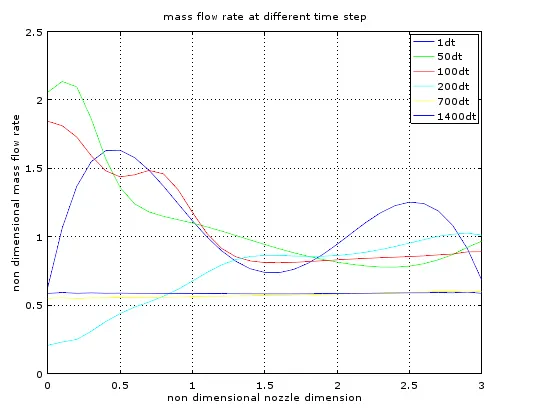
  %% plot for non dimensional mass flow rate

  figure(1)
  hold on
  if k==1
      plot(x,m)
    hold on
    elseif k ==50
        plot(x,m,'g')
      hold on
      elseif k == 100
          plot(x,m,'r')
        hold on
        else if k==200
              plot(x,m,'c')
         hold on
         elseif k==700
                plot(x,m,'y')
          elseif k== 1400
                plot(x,m)
           grid on;
           xlabel('non dimensional nozzle dimension')
           ylabel('non dimensional mass flow rate')
           legend('1dt','50dt','100dt','200dt','700dt','1400dt')
           title('mass flow rate at different time step')
       end
 end
 toc;
end
conservative:
function [v_c,rho_c,t_c,m_c,M_c,p_c,v_t,rho_t,t_t,m_t,M_t,p_t,v_res_c,rho_res_c,t_res_c] = conservative_form(x,n,gamma,nt,dx,a)
%input variables
L=3;
n=61;
x=linspace(0,3,n);
dx=x(2)-x(1);
c=0.5;

%initial conditions of the non dimensional numbers
%x,rho,v,a are non dimensional numbers
a= 1+2.2*(x-1.5).^2;

%initial conditions
for i=1:n
      if (x(i)>=0 &&  x(i)<=0.5)
       rho_c(i)=1;
        t_c(i)=1;
      elseif (x(i)>=0.5 && x(i)<=1.5)
          rho_c(i)=1-0.366*(x(i)-0.5);
          t_c(i)=1-0.167*(x(i)-0.5);
      elseif (x(i)>=1.5  &&  x(i)<=3.5)
          rho_c(i) = 0.634-0.3879*(x(i)-1.5);
          t_c(i) = 0.833-0.3507*(x(i)-1.5);
      end
  end


%assuming steady state flow for the initial condition
  v_c = 0.59./(rho_c.*a);
  gamma = 1.4;
  throat = find(a==1);


  %solution vector parameters
  pr = rho_c.*t_c;
  u1 = rho_c.*a;
  u2 = rho_c.*a.*v_c;
  u3 = u1.*((t_c./(gamma-1))+((gamma/2).*(v_c.^2)));

  %calculation of time step
  dt = min (c.*(dx./((t_c.^0.5)+v_c)));

  % number of time cycle
    nt=1400;

    %time loop
  for k=1:nt

      %copy of solution vectors
        u1_old =u1;
        u2_old =u2;
        u3_old =u3;


        % pure form of flux terms
        f1 =u2;
        term = (((gamma-1)/gamma)*(u3-((gamma/2)*((u2.^2)./u1))));
        f2 = ((u2.^2)./u1)+term;
        f3 =((gamma*u2.*u3)./u1)-(gamma*(gamma-1)*(u2.^3))./(2*u1.^2);

        %predictor method
        for i=2:n-1


              df1dx(i) = (f1(i+1)-f1(i))/dx;
              df2dx(i) = (f2(i+1)-f2(i))/dx;
              df3dx(i) = (f3(i+1)-f3(i))/dx;

              dadx(i) = (a(i+1)-a(i))/dx;
              j2(i) = (1/gamma)*(rho_c(i)*t_c(i))*dadx(i);

              %continuity equation
              du1dt_p(i) = -df1dx(i);

              %momentum equation
              du2dt_p(i) =-df2dx(i) + j2(i);

              % energy equation
              du3dt_p(i) = -df3dx(i);

              %solution update
              u1(i) = u1(i) + du1dt_p(i)*dt;
              u2(i) = u2(i) + du2dt_p(i)*dt;
              u3(i) = u3(i) + du3dt_p(i)*dt;

        end


      %decoding primitive terms to initialize the corrector step
      rho_c = u1./a;
      v_c = u2./u1;
      t_c = (gamma -1)*((u3./u1)-((gamma*v_c.^2)/2));

      % "pure" form of the flux terms for the corrector step
      f1=u2;
      term1 = (((gamma-1)/gamma)*(u3-(gamma*u2.^2)./(2*u1)));
      f2=((u2.^2)./u1)+term1;
      f3 = ((gamma*u2.*u3)./u1)-(gamma*(gamma-1)*(u2.^3))./(2*u1.^2);

      %corrector method
      for i= 2:n-1

            df1dx(i) = (f1(i)-f1(i-1))/dx;
            df2dx(i) = (f2(i) - f2(i-1))/dx;
            df3dx(i) = (f3(i) -f3(i-1))/dx;

            dadx1(i) = (a(i)-a(i-1))/dx;
            j3(i) = (1/gamma)*(rho_c(i)*t_c(i))*dadx1(i);

            %continuity equation
            du1dt_c(i) = -df1dx(i);

            %momentum equation
            du2dt_c(i) = -df2dx(i) + j3(i);

            %energy  equation
            du3dt_c(i) = -df3dx(i);

         end

         %average derivative
         du1dt = 0.5*(du1dt_p + du1dt_c);
         du2dt = 0.5*(du2dt_p + du2dt_c);
         du3dt = 0.5*(du3dt_p + du3dt_c);

         % final solution update
         for j= 2:n-1
              u1(j) = u1_old(j) + du1dt(j)*dt;
              u2(j) = u2_old(j) + du2dt(j)*dt;
              u3(j) = u3_old(j) + du3dt(j)*dt;
            end

            %apply the boundary conditions

            %inlet

            %u1 value remains same, because rho is not a floating variable and also doesnot change with time
            u1(1) =rho_c(1)*a(1);

            %velocity is the floating primitive term, which can be calculated by extrapolating u2
            u2(1) =2*u2(2) - u2(3);

            %floating variable v, is calculated for every time step
            v_c(1) = u2(1)/u1(1);

            %updating u3
            u3(1) = u1(1)*((t_c(1)/(gamma-1))+((gamma/2)*v_c(1)^2));

            %outlet
            u1(n) =2*u1(n-1) -u1(n-2);
            u2(n) = 2*u2(n-1) - u2(n-2);
            u3(n) = 2*u3(n-1) -u3(n-2);

            %decoding primitive terms
            rho_c = u1./a;
            v_c = u2./u1;
            t_c = (gamma-1)*((u3./u1)-((gamma*v_c.^2)/2));


            %calculating solutions
            m_c = rho_c.*v_c.*a;
            M_c = v_c./((t_c).^0.5);
            p_c = rho_c.*t_c;

            %throat values
            rho_t(k) = rho_c(throat);
            t_t(k) = t_c(throat);
            p_t(k) = p_c(throat);
            M_t(k) = M_c(throat);
            v_t(k) = v_c(throat);
            m_t(k) = m_c(throat);

            %residual convergence

            rho_res_c(k) = du1dt(throat);
            t_res_c(k) = du2dt(throat);
            v_res_c(k) = du3dt(throat);

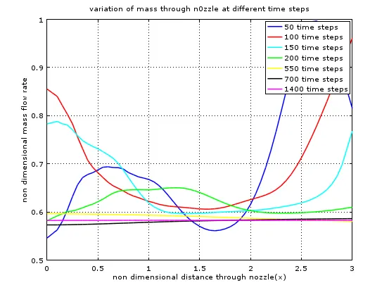
            %plotting mass flow rate at different time steps
            figure(2);
            if k == 50
              plot(x,m_c, 'b', 'linewidth', 1.5)
            hold on
                elseif k == 100
                    plot(x,m_c, 'r', 'linewidth', 1.5)
                  hold on
                elseif k == 150
                    plot(x,m_c, 'c', 'linewidth', 1.5)
                  hold on
                elseif k == 200
                    plot(x,m_c, 'g', 'linewidth', 1.5)
                  hold on
                elseif k == 550
                    plot(x,m_c, 'y', 'linewidth', 1.5)
                  hold on
                 elseif k == 700
                    plot(x,m_c, 'k', 'linewidth', 1.5)
                  hold on
                  elseif k == 1400
                    plot(x,m_c, 'm', 'linewidth', 1.5)

                  grid on
                  ylabel('non dimensional mass flow rate')
                 xlabel('non dimensional distance through nozzle(x)')
                 title ('variation of mass through n0zzle at different time steps')
                 legend({'50 time steps', '100 time steps', '150 time steps', '200 time steps', '550 time steps', '700 time steps', '1400 time steps'});
               end
           end
            toc;

        end