Week 7 - Simulation of a 1D Super-sonic nozzle flow simulation using Macormack Method
Aim:
To simulate 1D Super-sonic nozzle flow using the MacCormack Method with both the conservation and non-conservation forms of the governing equations
Problem Description:
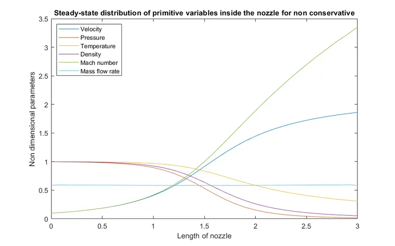
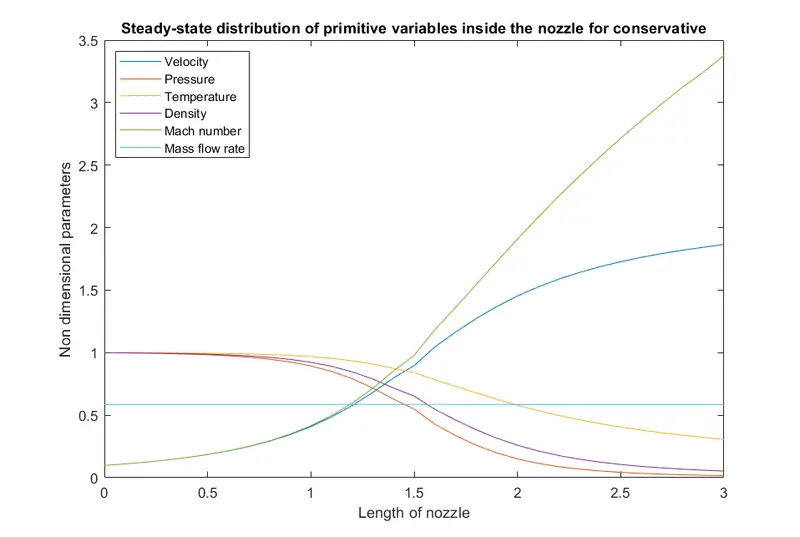
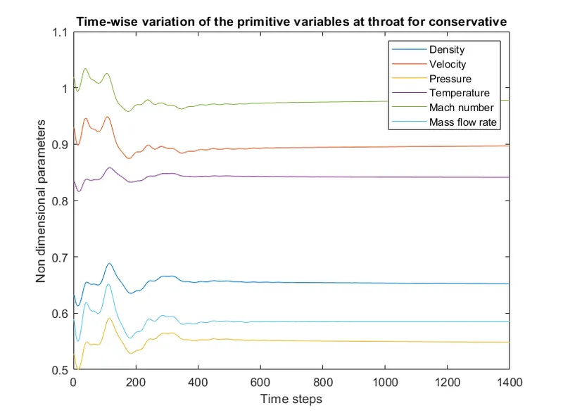
The flow in a nozzle is to be simulated and get the values of primitives which are Velocity, Pressure, Temperature, Density, Mach number and Mass flow rate.
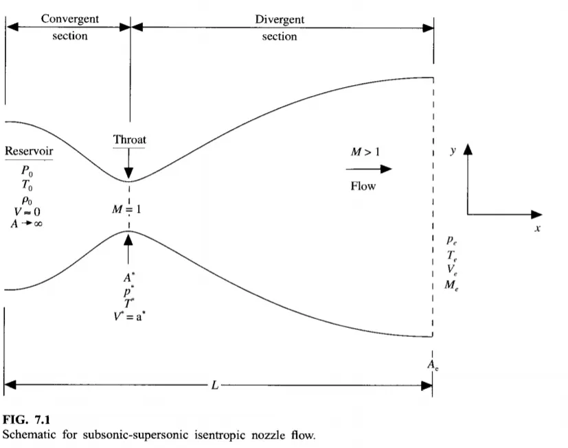
Formulation:
- For Non-Dimensional variables:
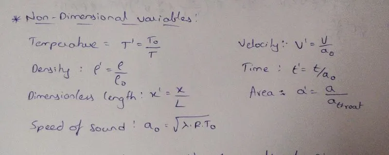
Main Code:
close all
clear all
clc
%% Initalization
l = 3; % length of the nozzle
n = [31 61]; % Number of grid points
c = 0.5; % CFL number
nt = 1:1400; % Time step

for i = 1:length(n)
    %% Solving using Conservative and Non-Conservative form
    x=linspace(0,l,n(i));
    [m_non_con,m_throat_non_con]=non_conservative(l,n(i),nt,c);
    [m_con,m_throat_con]=conservative(l,n(i),nt,c);

    figure(7)
    subplot(2,1,1)
    plot(x,m_con,x,m_non_con)
    xlabel('Length of nozzle')
    ylabel('Mass flow rate')
    legend('Conservative form','Non-Conservative form')
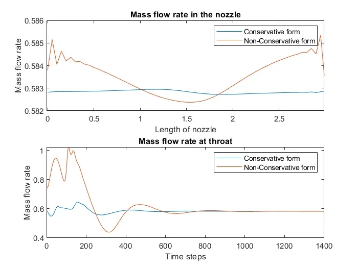
    title('Mass flow rate in the nozzle')

    subplot (2,1,2)
    plot(nt,m_throat_con,nt,m_throat_non_con)
    xlabel('Time steps')
    ylabel('Mass flow rate')
    legend('Conservative form','Non-Conservative form')
    title('Mass flow rate at throat')
    %% Grid independency test
    figure(8)
    subplot (2,1,1)
    plot(x,m_con)
    hold on
    xlabel('Length of nozzle')
    ylabel('Mass flow rate')
    legend('With 31 nodes','With 61 nodes')
    title('Grid independence test along the nozzle for conservative')
    subplot (2,1,2)
    plot(x,m_non_con)
    hold on
    xlabel('Length of nozzle')
    ylabel('Mass flow rate')
    legend('With 31 nodes','With 61 nodes')
    title('Grid independence test along the nozzle for non-conservative')

    figure(9)
    subplot (2,1,1)
    plot(nt,m_throat_con)
    hold on
    xlabel('Time steps')
    ylabel('Mass flow rate')
    legend('With 31 nodes','With 61 nodes')
    title('Grid independence test at throat point for conservative')
    subplot (2,1,2)
    plot(nt,m_throat_non_con)
    hold on
    xlabel('Time steps')
    ylabel('Mass flow rate')
    legend('With 31 nodes','With 61 nodes')
    title('Grid independence test at throat point for non-conservative')
end
Non-Conservative form:
Formulation:
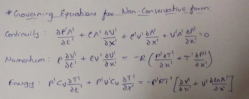
Conditions:
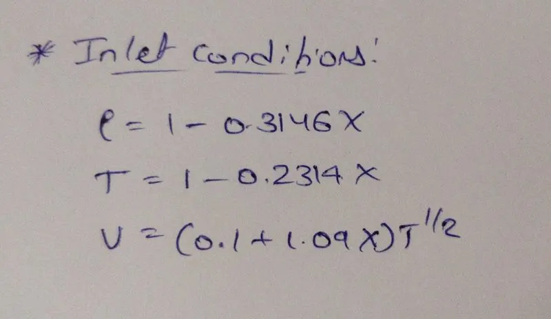
Function Code:
function [m_non_con,m_throat_non_con]=non_conservative(l,n,nt,c)

%% Creating grid
x=linspace(0,l,n);
dx=x(2)-x(1);
% initial conditions rho, a, v, T, mfr, M, p
%% Initialization
a= 1+2.2*(x-1.5).^2;     % Area of nozzle
throat = find(a==1);     % To find node where area is unity
g = 1.4;                 % Gamma value
rho = 1-0.3146*x;
t= 1-0.2314*x;
v=(0.1+1.09*x).*t.^0.5;
a= 1+2.2*(x-1.5).^2;
M= v./(t.^0.5); % Mach number
m = rho.*a.*v; % Mass flow rate
p=rho.*t;
% Finding dt value
for z=1:31
    u=(t(z))^(1/2);
    dt(z) = c*dx/(u + v(z));
end
dt=min(dt);

for i = 1:length(nt)
    % To store initial values
    rho_old = rho;
    T_old = t;
    v_old = v;
    for j=2:n-1
        %% Predictor step
        drho_dx = (rho(j+1)-rho(j))/dx;
        dv_dx = (v(j+1)-v(j))/dx;
        dT_dx = (t(j+1)-t(j))/dx;
        da_dx = (log(a(j+1))-log(a(j)))/dx;
        drho_dt_p(j) = -rho(j)*dv_dx - rho(j)*v(j)*da_dx - v(j)*drho_dx;
        dv_dt_p(j) = -v(j)*dv_dx - (1/g)*(dT_dx + (t(j)/rho(j))*drho_dx);
        dT_dt_p(j) = -v(j)*dT_dx - (g-1)*t(j)*(dv_dx + v(j)*da_dx);
        %updating primitives
        v(j) = v_old(j) + dv_dt_p(j)*dt;
        rho(j) = rho_old(j) + drho_dt_p(j)*dt;
        t(j) = T_old(j) + dT_dt_p(j)*dt;
        %% Corrector step
        drho_dx = (rho(j)-rho(j-1))/dx;
        dv_dx = (v(j)-v(j-1))/dx;
        dT_dx = (t(j)-t(j-1))/dx;
        da_dx = (log(a(j))-log(a(j-1)))/dx;
        drho_dt_c(j) = -rho(j)*dv_dx - rho(j)*v(j)*da_dx - v(j)*drho_dx;
        dv_dt_c(j) = -v(j)*dv_dx - (1/g)*(dT_dx + (t(j)/rho(j))*drho_dx);
        dT_dt_c(j) = -v(j)*dT_dx - (g-1)*t(j)*(dv_dx + v(j)*da_dx);
    end
    %% Caclulating avg gradient
    drho_dt_avg = 0.5*(drho_dt_p + drho_dt_c);
    dv_dt_avg = 0.5*(dv_dt_p + dv_dt_c);
    dT_dt_avg = 0.5*(dT_dt_p + dT_dt_c);

    for k = 2:n-1
        rho(k) = rho_old(k) + drho_dt_avg(k)*dt;
        v(k) = v_old(k) + dv_dt_avg(k)*dt;
        t(k) = T_old(k) + dT_dt_avg(k)*dt;
    end
    %% Boundary conditions
    v(1) = 2*v(2)-v(3); % entry
    v(n) = 2*v(n-1)-v(n-2); %exit
    rho(n) = 2*rho(n-1)-rho(n-2);
    t(n) = 2*t(n-1)-t(n-2);

    %% Getting Final Primitives
    p = rho.*t;
    M= v./t.^0.5;
    error(k) =  abs(v(k)-v(k-1));
    m= rho.*a.*v;

    %% To find values at throat point
    m_thr(i)=m(throat);
    t_thr(i) = t(throat);
    rho_thr(i) = rho(throat);
    M_thr(i) = M(throat);
    v_thr(i) = v(throat);
    p_thr(i) = p(throat);
    error_thr(i)=error(throat);

    if n==31
        for h=[1:50:201 700]
            if h==i
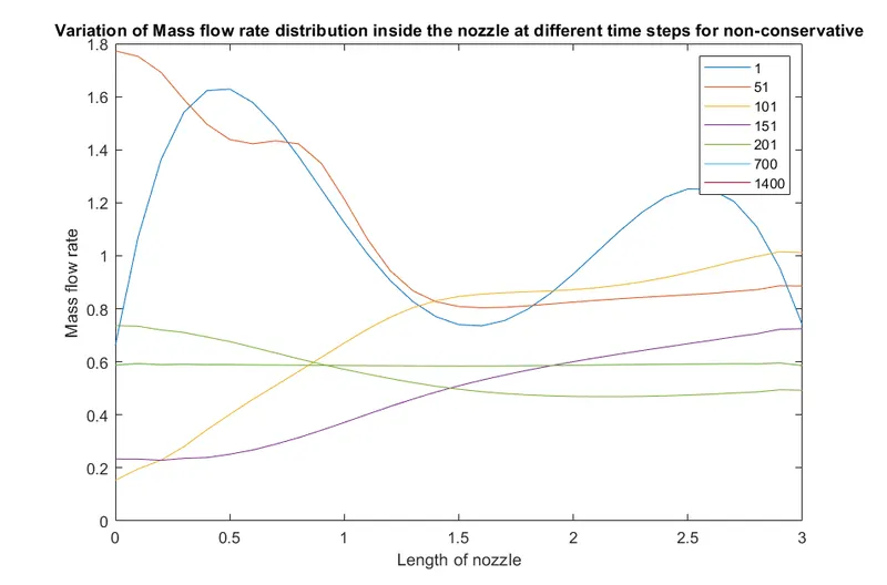
                figure(1)
                plot(x,m)
                hold on
                title ('Variation of Mass flow rate distribution inside the nozzle at different time steps for non-conservative')
                xlabel('Length of nozzle')
                ylabel('Mass flow rate')
            elseif i==1400
                plot(x,m)
                legend('1','51','101','151','201','700','1400')
            end
        end
    end

end
if n==31
    figure(2)
    plot(x,v,x,p,x,t,x,rho,x,M,x,m)
    xlabel('Length of nozzle')
    ylabel('Non dimensional parameters')
    legend('Velocity','Pressure','Temperature','Density','Mach number','Mass flow rate')
    title('Steady-state distribution of primitive variables inside the nozzle for non conservative')

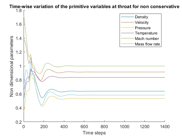
    figure (3)
    hold on
    plot(nt,rho_thr)
    plot(nt,v_thr)
    plot(nt,p_thr)
    plot(nt,t_thr)
    plot(nt,M_thr)
    plot(nt,m_thr)
    xlabel('Time steps')
    ylabel('Non dimensional parameters')
    legend('Density','Velocity','Pressure','Temperature','Mach number','Mass flow rate')
    title('Time-wise variation of the primitive variables at throat for non conservative')
end
m_non_con=m;
m_throat_non_con=m_thr;
end
Conservative form:
Formulation:
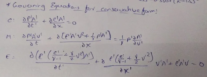
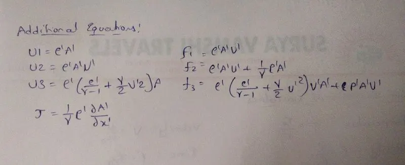
Conditions:
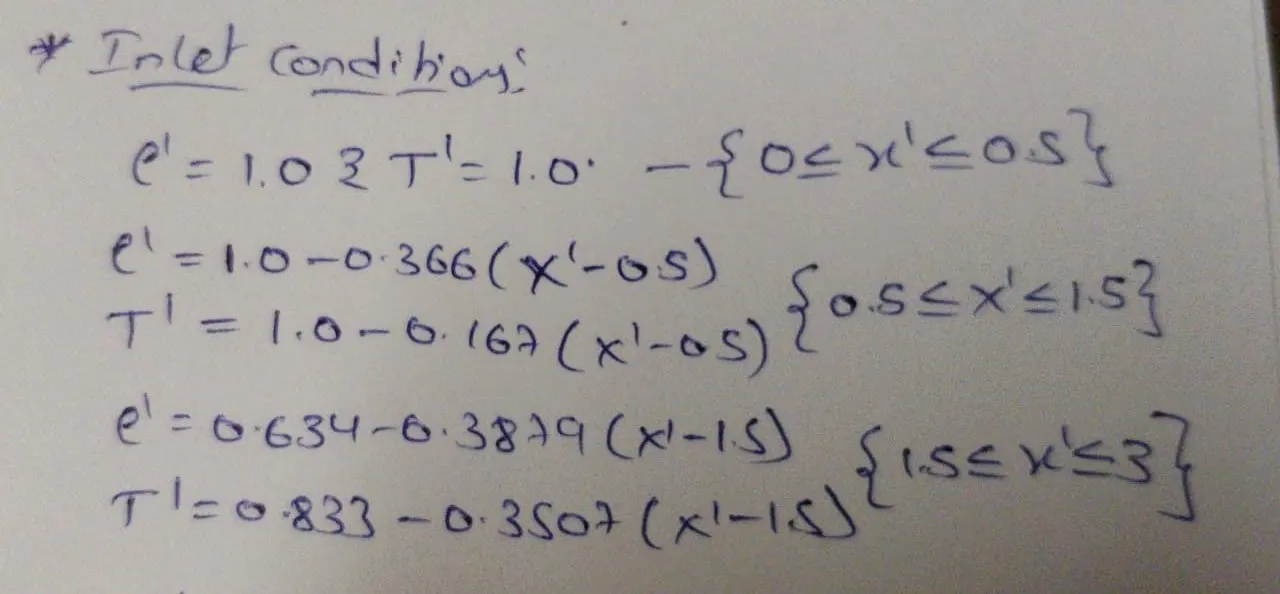
Function Code:
function [m_con,m_throat_con]=conservative(l,n,nt,c)

%% Creating grid
x=linspace(0,l,n);
dx=x(2)-x(1);
%% Initialization
a= 1+2.2*(x-1.5).^2;     % Area of nozzle
throat = find(a==1);     % To find node where area is unity
g = 1.4;                 % Gamma value
for k=1:length(x)
    if (x(k)<=0.5)
        rho(k) = 1;
        t(k) = 1;
    elseif (x(k)>0.5) && (x(k)<=1.5)
        rho(k) = 1-0.366*(x(k)-0.5);
        t(k)= 1-0.167*(x(k)-0.5);
    elseif (x(k)>1.5) && (x(k)<=3.5)
        rho(k) = 0.634-0.3879*(x(k)-1.5);
        t(k)= 0.833-0.3507*(x(k)-1.5);
    end
end

%% Source terms
u1 = rho.*a;
u2 = 0.59*ones(1,n);
v=u2./u1;
u3 = u1.*((t./(g-1))+(g/2).*v.^2);

M= v./(t.^0.5);  % Mach number
m = rho.*a.*v;   % Mass flow rate
p=rho.*t;        % Pressure
% Finding dt value
for z=1:31
    u=(t(z))^(1/2);
    dt(z) = c*dx/(u + v(z));
end
dt=min(dt);

for i = 1:length(nt)
    % To store initial values
    u1_old = u1;
    u2_old = u2;
    u3_old = u3;

    for j=2:n-1

        f1 = u2;
        f2 = ((u2.^2)./u1)+((g-1)/g)*(u3-((g/2)*(u2.^2)./u1));
        f3 = ((g.*u2.*u3)./u1) - ((g*(g-1)/2)*(u2.^3)./(u1.^2));

        j1 = (1/g)*rho(j)*t(j)*((a(j+1)-a(j))/dx);
        %% Predictor step
        du1_dt_p(j)= -(f1(j+1)-f1(j))/dx;
        du2_dt_p(j)= -(f2(j+1)-f2(j))/dx + j1;
        du3_dt_p(j)= -(f3(j+1)-f3(j))/dx;

        u1(j) = u1_old(j) + du1_dt_p(j)*dt;
        u2(j) = u2_old(j) + du2_dt_p(j)*dt;
        u3(j) = u3_old(j) + du3_dt_p(j)*dt;

        rho=u1./a;
        t=(g-1).*(u3./u1-(g/2).*(u2./u1).^2);

        f1=u2;
        f2=u2.^2./u1+((g-1)/g).*(u3-(g/2)*u2.^2./u1);
        f3=g.*u2.*u3./u1-0.5*g*(g-1).*u2.^3./u1.^2;

        j2 = (1/g)*(rho(j)*t(j)*(a(j)-a(j-1))/dx);
        %% Corrector step
        du1_dt_c(j) = -(f1(j)-f1(j-1))/dx;
        du2_dt_c(j) = -(f2(j)-f2(j-1))/dx + j2;
        du3_dt_c(j) = -(f3(j)-f3(j-1))/dx;
    end
    %% Caclulating avg gradient
    du1_dt_avg = 0.5*(du1_dt_p + du1_dt_c);
    du2_dt_avg = 0.5*(du2_dt_p + du2_dt_c);
    du3_dt_avg = 0.5*(du3_dt_p + du3_dt_c);

    for k = 2:n-1
        u1(k) = u1_old(k) + du1_dt_avg(k)*dt;
        u2(k) = u2_old(k) + du2_dt_avg(k)*dt;
        u3(k) = u3_old(k) + du3_dt_avg(k)*dt;
    end

    u1(1) = a(1);
    u2(1) = 2*u2(2)-u2(3);
    u3(1) = u1(1)*(t(1)/(g-1) + (g*(u2(1)/u1(1))^2)/2);

    u1(n) = 2*u1(n-1)-u1(n-2);
    u2(n) = 2*u2(n-1)-u2(n-2);
    u3(n) = 2*u3(n-1)-u3(n-2);

    %% Getting Final Primitives
    rho = u1./a;
    v = u2./u1;
    t=(g-1).*(u3./u1-(g/2).*(u2./u1).^2);
    p = rho.*t;
    M= v./t.^0.5;
    error(k) =  abs(v(k)-v(k-1));
    m= u2;
    %% To find values at throat point
    m_throat(i)=m(throat);
    t_throat(i) = t(throat);
    rho_throat(i) = rho(throat);
    M_throat(i) = M(throat);
    v_throat(i) = v(throat);
    p_throat(i) = p(throat);
    error_throat(i)=error(throat);

    %% Ploting only for 31 nodes configuration
    if n==31 % This can be changed to get plots at different no of nodes
        for k=[1:50:201 700]
            if k==i
                figure(4)
                plot(x,m)
                hold on
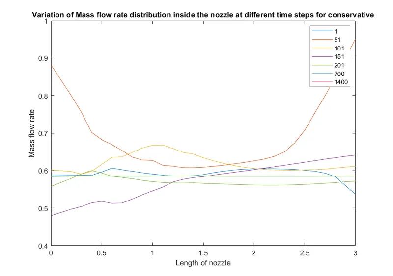
                title ('Variation of Mass flow rate distribution inside the nozzle at different time steps for conservative')
                xlabel('Length of nozzle')
                ylabel('Mass flow rate')
            elseif i==1400
                plot(x,m)
                legend('1','51','101','151','201','700','1400')
            end
        end
    end

end
if n==31
    figure(5)
    plot(x,v,x,p,x,t,x,rho,x,M,x,m)
    xlabel('Length of nozzle')
    ylabel('Non dimensional parameters')
    legend('Velocity','Pressure','Temperature','Density','Mach number','Mass flow rate')
    title('Steady-state distribution of primitive variables inside the nozzle for conservative')

    figure (6)
    plot(nt,rho_throat)
    hold on
    plot(nt,v_throat)
    plot(nt,p_throat)
    plot(nt,t_throat)
    plot(nt,M_throat)
    plot(nt,m_throat)
    xlabel('Time steps')
    ylabel('Non dimensional parameters')
    legend('Density','Velocity','Pressure','Temperature','Mach number','Mass flow rate')
    title('Time-wise variation of the primitive variables at throat for conservative')
end
m_con=m;
m_throat_con=m_throat;

end
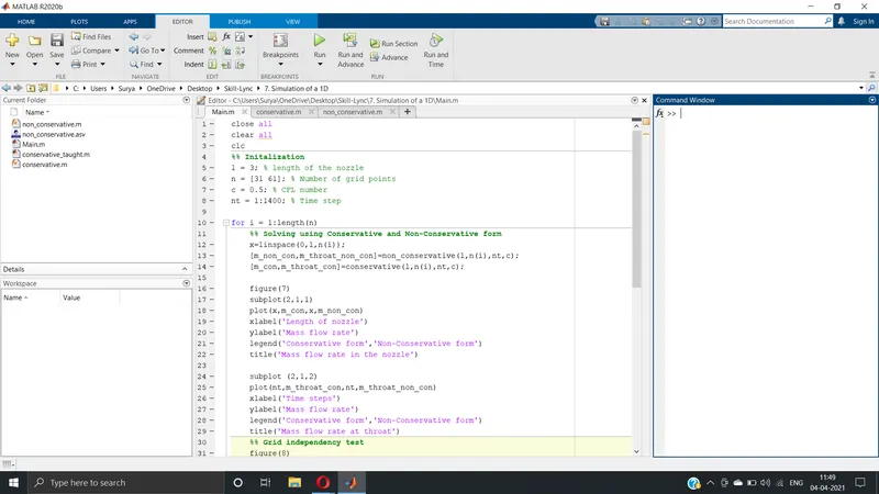
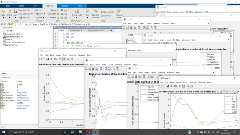
Screenshots:
Results:
Non-Conservative form:
Conservative form:
Comparison of Normalized mass flow rate distributions of both forms:
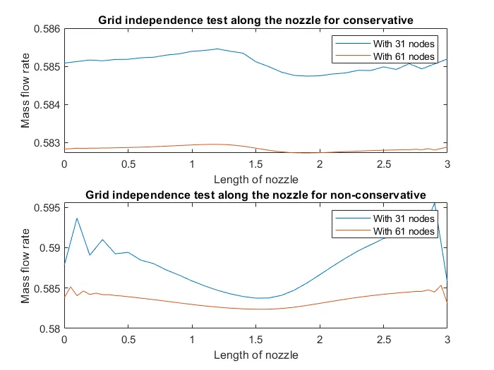
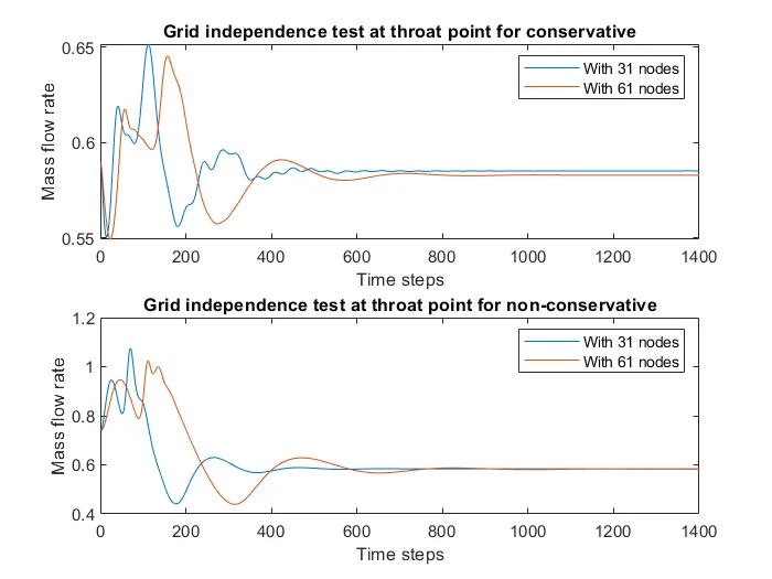
Grid Independence Test:
Conclusion:
- All the plots requested are obtained.
- There is a difference between solutions obtained with conservative and non-conservative forms.
- Also, grid size must also be taking into consideration as there is a slight difference in the solution whereas it also affects the computing time and resources.