Week 7 - Simulation of a 1D Super-sonic nozzle flow simulation using Macormack Method
SIMULATION OF 1D SUPER-SONIC NOZZLE FLOW SIMULATION USING MACORMACK METHOD:
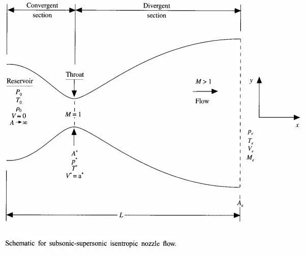
Consider the steady,isentropic flow through a converegnt-divergent nozzle. The flow at the inlet to the nozzlee comes from a reservoir where th pressure and temperature are denoted by `p_0,T_0`respectively.Cross-sectional area of reservoir is large(A-infinity),hence velocity is very small(v-0).`p_0,T_0`are the stagnation values.The flow expands isentropically to supersonic speeds at the nozzle exit where the exit pressure, temperature,velocity and mach number are denoted by `p_e,T_e,V_e,M_e` respectively.The flow is locally subsonic in the convergent section of the nozzle,sonic flow(M=1)at the throat means local velocity at this location is equal to the local speed of the sound.Use asterisk to denote sonic flow values p-p*,T-T*,V=V=a*
Flow field is two-dimensional(flow varies in xy space),assume that flow properties vary only with x and uniform flow properties across any give cross section.Such flow is called quasi-one-dimensional flow.
Conservative and non-conservative are differ only in numerical discretization.Conservative are more accurate.Conservative tend to work well when discontinuities exist in the domain.
For the nozzle flows,the flow field variables are frequently expressed in terms of non dimensional variables where flow variables are referenced to their reservoir values.Such as
`T'=T/T_0,rho'=rho/rho_0,a_0=sqrt(gammaRT_0),V'=V/a_0,t'=t/(L/a_0),A'=A/A^*`
GOVERNING EQUATION OF NON-CONSERVATIVE FORM:
Continuity Equation:
`(delp)/(delt)=-rho(delv)/dx-delv(del(lnA))/(delx)-v(delrho)/(delx)`
Momentum Equation:
`(delv)/(delt)=-v(delv)/(dx)-1/gamma((delT)/(delx)+T/rho(delrho)/(delx))`
Energy Equation:
`(delT)/(delt)=-v(delT)/(delx)-(gamma-1)T'((delv)/(delx)+v'(del(lnA'))/(dx))`
Equations are splitted to avoid human error.So defined the elements of the solution as solution vector U,the flux vector F,the source term J
MACCORMACK METHOD:
MacCormack's technique is described as two-step predictor-corrector method.Predictor sequence is used with forward differences and corrector sequence is used with backward differences.It has the same accuracy as the Lax-Wndroff method.Here MacCormack method is much easier to apply,because ther is no need to evaluate second time derivative as the case for Lax-Wendroff method.Because those equation represent large number of additional calculations(lot of algebraic equation).
Here we will setup a time-marching finite difference solution for the quasi-one-dimensional nozzle flow.
Predictor Step:
Replace the spatial derivatives on the right hand side with forward differences.
`(dv)/(dx)=(v(i+1)-v(i))/dx`
`(drho)/(dx)=(rho(i+1)-rho(i))/dx`
`(dt)/(dx)=(t(i+1)-t(i))/dx`
`(dloga)/(dx)=(log(a(i+1))-log(a(i)))/dx`
Corrector Step:
Replace the spatial erivatives with backward difference.
`(dv)/(dx)=(v(i)-v(i-1))/dx`
`(drho)/(dx)=(rho(i)-rho(i-1))/dx`
`dt/(dx)=(t(i)-t(i-1))/dx`
`(dloga)/(dx)=(log(a(i))-log(a(i-1)))/dx`
Initial Conditions:
`rho=1-0.3146x`
`t=1-0.2314x`
`v=(0.1+1.09x)sqrt(t)`
`a=1+2.2(x-1.5)^2`
To find average of predictor and corrector step:
`((drho)/(dt))_(avg)=0.5((drho)/dt_p+(drho)/dt_c)`
`((dv)/(dt))_(avg)=0.5((dv)/dt_p+(dv)/dt_c)`
`((dt)/dt)_(avg)=0.5((dt)/dt_p+dt/dt_c)`
GOVERNING EQUATION OF CONSERVATIVE FORM:
Continuity Equation:
`F_1=U_2`
`U_2=rho'A'V'`
Momentum Equation:
`F_2=(U_2^2/U_1)+((gamma-1)/gamma)(U_3-gamma/2U_2^2/U_1^2)`
`U_1=rho'A'`
Energy Equation:
`F_3=gamma(U_2U_3)/U_1-gamma(gamma-1)/2U_3^2/U_1^2`
`J_2=(gamma-1)/gamma(U_3-gamma/2(U_2^2/U_1))((del(lnA'))/(dx'))`
Initial Conditions:
For `0lexle0.5`
`rho=1;T=1`
For `0.5lexle1.5`
`rho=1-0.366(x-0.5)`
`T=1-0.167(x-0.5)`
For `1.5lexle3.5`
`rho=0.634-0.3879(x-1.5)`
`T=0.833-0.3507(x-1.5)`
To find average of predictor and corrector step:
`((delU_1)/dt)_(avg)=0.5((delU_1)/(delt_p)+(delU_1)/(delt_c))`
`((delU_2)/dt)_(avg)=0.5((delU_2)/(delt_p)+(delU_2)/(delt_c))`
`((delU_3)/dt)_(avg)=0.5((delU_3)/(delt_p)+(delU_3)/(delt_c))`
Solution update
`U_1^2=U_1+((delU_1)/dt)_(avg)`
`U_2^2=U_2+((delU_1)/dt)_(avg)`
`U_3^2=U_3^1+((delU_1)/dt)_(avg)`
Grid points= 30
Inlet Condition:
`U_1(1) = a(1);`
`U_2(1) = 2*U_2(2)-U_2(3)`
`v(1) = (U_2(1))/(U_1(1)`
`U_3(1) = U_1(1)*(T'(1)/(gamma-1)+ (gamma/2)*v(1)^2)`
Outlet Condition:
`U_1(n) = 2*U_1(n-1)-U_1(n-2)`
`U_2(n) = 2*U_2(n-1)-U_2(n-2)`
`U_3(n) = 2*U_3(n-1)-U_3(n-2)`
Mass flow rate `m = rhoAv`
Mach Number `M = v/sqrt(t)`
Pressure`p = rhot`
MAIN PROGRAM:
clear all
close all
clc
%inputs
n=31;
x=linspace(0,3,n);
dx=x(2)-x(1);
gamma=1.4;
nt = 1400;

[m_nc] = supersonic_nozzle(x,dx,n,gamma,nt);
[m_c] = supersonic_nozzle_conservation(x,dx,n,gamma,nt);


figure(8)
plot(x,m_nc,x,m_c)
title('Normalized mass flow rate distributions of both forms')
xlabel('length of the nozzle')
ylabel('mass flow rate')
legend('non conservation form','conservation form')
FUNCTION PROGRAM FOR NON-CONSERVATIOM FORM:
function m = supersonic_nozzle(x,dx,n,gamma,nt)


%calculation of initial profiles
rho=1-0.3146*x;
t=1-0.2314*x;
v=(0.1+1.09*x).*sqrt(t);
a=1+2.2*(x-1.5).^2;

%timesteps
dt=0.0201;
%outer time loop
for k=1:nt
    rho_old = rho;
    v_old = v;
    t_old = t;
    %predictor method
    for i=2:n-1
        dvdx=(v(i+1)-v(i))/dx;
        drhodx=(rho(i+1)-rho(i))/dx;
        dtdx=(t(i+1)-t(i))/dx;
        dlogadx=(log(a(i+1))-log(a(i)))/dx;

        %continuity equation
        drhodt_p(i)=-rho(i)*dvdx-rho(i)*v(i)*dlogadx-v(i)*drhodx;

        %momentum equation
        dvdt_p(i)=-v(i)*dvdx-(1/gamma)*(dtdx+(t(i)/rho(i))*drhodx);

        %Energy equation
        dtdt_p(i)=-v(i)*dtdx-(gamma-1)*t(i)*(dvdx+v(i)*dlogadx);
        %solution update
        rho(i)=rho(i)+drhodt_p(i)*dt;
        v(i)=v(i)+dvdt_p(i)*dt;
        t(i)=t(i)+dtdt_p(i)*dt;
    end
    %corrector method
    for i=2:n-1
        dvdx=(v(i)-v(i-1))/dx;
        drhodx=(rho(i)-rho(i-1))/dx;
        dtdx=(t(i)-t(i-1))/dx;
        dlogadx=(log(a(i))-log(a(i-1)))/dx;

        %continuity equation
        drhodt_c(i)=-rho(i)*dvdx-rho(i)*v(i)*dlogadx-v(i)*drhodx;

        %momentum equation
        dvdt_c(i)=-v(i)*dvdx-(1/gamma)*(dtdx+(t(i)/rho(i))*drhodx);

        %Energy equation
        dtdt_c(i)=-v(i)*dtdx-(gamma-1)*t(i)*(dvdx+v(i)*dlogadx);
    end


    %compute avg time derivative
    drhodt=0.5*(drhodt_p+drhodt_c);
    dvdt=0.5*(dvdt_p+dvdt_c);
    dtdt=0.5*(dtdt_p+dtdt_c);

        %final solution update
    for j=2:n-1
        v(j)=v_old(j)+dvdt(j)*dt;
        rho(j)=rho_old(j)+drhodt(j)*dt;
        t(j)=t_old(j)+dtdt(j)*dt;
    end

    %Apply Boundary condition
    %inlet
    v(1)=2*v(2)-v(3);
    %outlet
    v(n)=2*v(n-1)-v(n-2);
    rho(n)=2*rho(n-1)-rho(n-2);
    t(n)=2*t(n-1)-t(n-2);

    m = rho.*a.*v;
    M = v./sqrt(t);
    p = rho.*t;


    rho_th(k) = rho(16);
    p_th(k) = p(16);
    t_th(k) = t(16);
    v_th(k) = v(16);
    M_th(k) = M(16);

    dvdt_th(k) = abs(dvdt(16));
    dtdt_th(k) = abs(dtdt(16));

    figure(4)
    title('Mass flow distribution')
    if k==1
        plot(x,m,'-k');
    end
    hold on
    if k==50
        plot(x,m);
    end
    if k==100
        plot(x,m);
    end
    if k==150
        plot(x,m);
    end
    if k==200
        plot(x,m);
    end
    if k==400
        plot(x,m);
    end
     if k==600
        plot(x,m);
     end
     if k==800
        plot(x,m);
     end
    xlabel('length of the nozzle')
    ylabel('mass flow')

end
    legend('1dt','50dt','100dt','150dt','200dt','400dt','600dt','800dt')
    figure(1)
    sgtitle('Quasi 1D nozzle flow:isentropic subsonic-supersonic solution')
    subplot(5,1,1)
    plot(x,v)
    xlabel('x')
    ylabel('v/v0')
    subplot(5,1,2)
    plot(x,t)
    xlabel('x')
    ylabel('t/t0')
    subplot(5,1,3)
    plot(x,rho)
    xlabel('x')
    ylabel('rho/rho0')
    subplot(5,1,4)
    plot(x,p)
    xlabel('x')
    ylabel('p/p0')
    subplot(5,1,5)
    plot(x,M)
    xlabel('x')
    ylabel('M')

    figure(2)
    sgtitle('Timewise variations of rho,t,p,M at the nozzle throat')
    subplot(5,1,1)
    plot(rho_th)
    xlabel('Number of time steps')
    ylabel('rho/rho0')
    subplot(5,1,2)
    plot(v_th)
    xlabel('Number of time steps')
    ylabel('v/v0')
    subplot(5,1,3)
    plot(p_th)
    xlabel('Number of time steps')
    ylabel('p/p0')
    subplot(5,1,4)
    plot(t_th)
    xlabel('Number of time steps')
    ylabel('t/t0')
    subplot(5,1,5)
    plot(M_th)
    xlabel('Number of time steps')
    ylabel('Mach number')


end
OBTAINED PLOT:
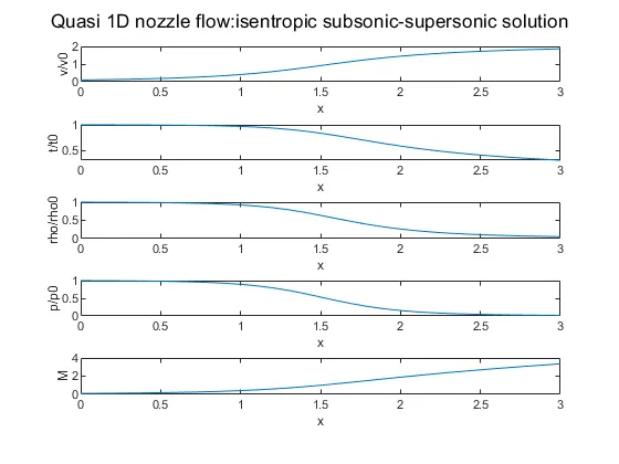
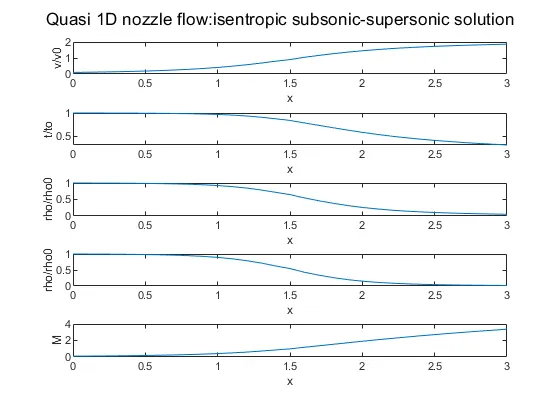
Steady-state distribution of primitive variables inside the nozzle
Variation of Mass flow rate distribution inside the nozzle at different time steps during the time-marching process
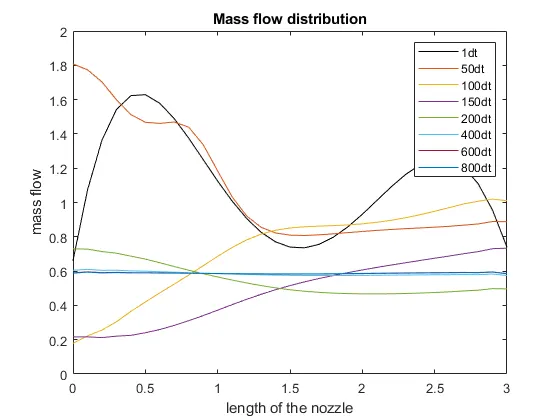
Mass flow rate vary from timestep-1 to timestep-800(dt-change in timestep).At the beginning time step of 1,heavy blows up of mass flow upto 1.8 and slowly redues and at time step 800,mass flows in linearly.
Time-wise variation of the primitive variables
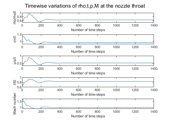
At 0 timestep represents initial condition and ends at 1400 timestep.density ratio,pressure ratio,temperature ratio starts increasing to right with larger changes velocity ratio and mach number decreases and after 300 timesteps ,steady state value is approached asymptomatically.It shows the solution converge.
FUNCTION PROGRAM FOR CONSERVATION FORM:
function m = supersonic_nozzle_conservation(x,dx,n,gamma,nt)
dt = 0.0267;
%initial conditions
for i=1:length(x)
if x(i)<=0.5
    rho(i) = 1;
    t(i) = 1;
end
if x(i)>0.5 && x(i)<=1.5
    rho(i) = 1 - 0.366*(x(i)-0.5);
    t(i) = 1 - 0.167*(x(i)-0.5);
end
if x(i)> 1.5
    rho(i) = 0.634 - 0.3879*(x(i)-1.5);
    t(i) = 0.833 - 0.3507*(x(i)-1.5);
end
end

a=1+2.2*(x-1.5).^2;
v = 0.59./(rho.*a);

%Source terms
u1 = rho.*a;
u2 = u1.*v;
u3 = u1.*(t/(gamma-1)+(gamma/2)*v.^2);

%time loop

for k=1:nt

u1_old = u1;
u2_old = u2;
u3_old = u3;


f1 = u2;
f2 = u2.^2./u1 + (gamma-1)/gamma*(u3 - 0.5*gamma*u2.^2./u1);
f3 = (gamma*u2.*u3)./u1 - (0.5*gamma*(gamma-1))*(u2.^3./u1.^2);

%Predictor

for i=2:n-1
   dadx = (a(i+1)-a(i))/dx;
   j2(i) = (1/gamma)*rho(i)*t(i)*dadx;

   du1dt_p(i) = -(f1(i+1)-f1(i))/dx;
   du2dt_p(i) = -(f2(i+1)-f2(i))/dx + j2(i);
   du3dt_p(i) = -(f3(i+1)-f3(i))/dx;

   u1(i) = u1(i) + du1dt_p(i)*dt;
   u2(i) = u2(i) + du2dt_p(i)*dt;
   u3(i) = u3(i) + du3dt_p(i)*dt;

end

rho = u1./a;
v = u2./u1;
t = (gamma-1)*((u3./u1)-(gamma/2)*(u2./u1).^2);

f1 = u2;
f2 = u2.^2./u1 + (gamma-1)/gamma*(u3 - 0.5*gamma*u2.^2./u1);
f3 = (gamma*u2.*u3)./u1 - (0.5*gamma*(gamma-1))*(u2.^3./u1.^2);

%Corrector

for j=2:n-1
   dadx = (a(j)-a(j-1))/dx;
   j2(j) = (1/gamma)*rho(j)*t(j)*dadx;

   du1dt_c(j) = -(f1(j)-f1(j-1))/dx;
   du2dt_c(j) = -(f2(j)-f2(j-1))/dx + j2(j);
   du3dt_c(j) = -(f3(j)-f3(j-1))/dx;

end
%compute avg time derivative
du1dt = 0.5*(du1dt_p + du1dt_c);
du2dt = 0.5*(du2dt_p + du2dt_c);
du3dt = 0.5*(du3dt_p + du3dt_c);

for j=2:n-1
u1(j) = u1_old(j) + du1dt(j)*dt;
u2(j) = u2_old(j) + du2dt(j)*dt;
u3(j) = u3_old(j) + du3dt(j)*dt;
end


%BC
%inlet
u1(1) = a(1);
u2(1) = 2*u2(2)-u2(3);
v(1) = u2(1)/u1(1);
u3(1) = u1(1)*(t(1)/(gamma-1)+ (gamma/2)*v(1)^2);
%outlet
u1(n) = 2*u1(n-1)-u1(n-2);
u2(n) = 2*u2(n-1)-u2(n-2);
u3(n) = 2*u3(n-1)-u3(n-2);

rho = u1./a;
v = u2./u1;
t = (gamma-1)*((u3./u1)-(gamma/2)*(u2./u1).^2);

m = rho.*a.*v;
M = v./sqrt(t);
p = rho.*t;

    rho_th(k) = rho(16);
    p_th(k) = p(16);
    t_th(k) = t(16);
    v_th(k) = v(16);
    M_th(k) = M(16);


    figure(7)
    title('Mass flow distribution')
    if k==1
        plot(x,m,'-k');
    end
    hold on
    if k==50
        plot(x,m);
    end
    if k==100
        plot(x,m);
    end
    if k==150
        plot(x,m);
    end
    if k==200
        plot(x,m);
    end
    if k==400
        plot(x,m);
    end
     if k==600
        plot(x,m);
     end
     if k==800
        plot(x,m);
     end
    xlabel('x')
    ylabel('mass flow')


end

legend('1dt','50dt','100dt','150dt','200dt','400dt','600dt','800dt')
    figure(5)
    sgtitle('Quasi 1D nozzle flow:isentropic subsonic-supersonic solution')
    subplot(5,1,1)
    plot(x,v)
    xlabel('x')
    ylabel('v/v0')
    subplot(5,1,2)
    plot(x,t)
    xlabel('x')
    ylabel('t/to')
    subplot(5,1,3)
    plot(x,rho)
    xlabel('x')
    ylabel('rho/rho0')
    subplot(5,1,4)
    plot(x,p)
    xlabel('x')
    ylabel('rho/rho0')
    subplot(5,1,5)
    plot(x,M)
    xlabel('x')
    ylabel('M')

    figure(6)
    sgtitle('Timewise variations of rho,t,p,M at the nozzle throat')
    subplot(5,1,1)
    plot(rho_th)
    xlabel('Number of time steps')
    ylabel('rho/rho0')
    subplot(5,1,2)
    plot(v_th)
    xlabel('Number of time steps')
    ylabel('v/a0')
    subplot(5,1,3)
    plot(p_th)
    xlabel('Number of time steps')
    ylabel('p/p0')
    subplot(5,1,4)
    plot(t_th)
    xlabel('Number of time steps')
    ylabel('t/t0')
    subplot(5,1,5)
    plot(M_th)
    xlabel('Number of time steps')
    ylabel('Mach number')
end
OBTAINED PLOT:
Steady-state distribution of primitive variables inside the nozzle
Variation of Mass flow rate distribution inside the nozzle at different time steps during the time-marching process
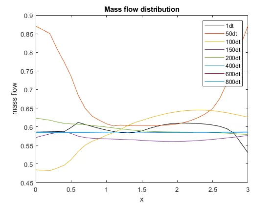
Mass flow rate vary from timestep-1 to timestep-800(dt-change in timestep).At the beginning time step of 1,heavy blows up of mass flow upto 0.87 and slowly redues and at time step 800,mass flows in linearly.
Time-wise variation of the primitive variables
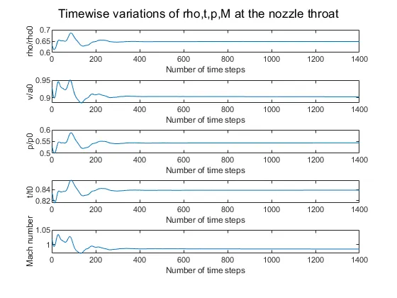
At 0 timestep represents initial condition and ends at 1400 timestep.density ratio,pressure ratio,temperature ratio starts increasing to right with larger changes velocity ratio and mach number decreases and after 200 timesteps ,steady state value is approached asymptomatically.It shows the solution converge.
RESULTS:
Comparison of Normalized mass flow rate distributions of both forms
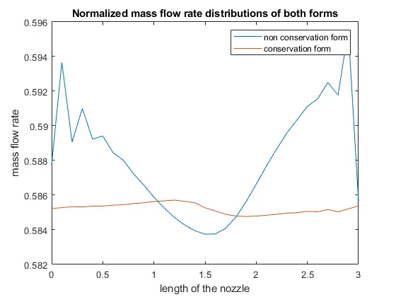
Conservation form gives a distribution that is much closer to constant while Non-conservation has sizeable variation with some oscillations at both inflow and outflow.
Steady state mass flow results obtained with conservation form is much closer to the exact analytical solution of 0.579
| Case | `rho^*/rho_0` | `T^*/T_0` | `p^*/p_0` | M |
| Exact Analytical Solution | 0.634 | 0.833 | 0.528 | 1.000 |
|
Non-Conservation form Numerical results n=31 |
0.6387 | 0.8365 | 0.5242 | 0.9994 |
|
Non-Conservation form Numerical results n=61 |
0.6377 | 0.8354 | 0.0.5327 | 0.9997 |
|
Conservation form Numerical results n=31 |
0.6486 | 0.8391 | 0.5442 | 0.9851 |
|
Conservation form Numerical results n=61 |
0.6376 | 0.8348 | 05322 | 1.0006 |
From the solution,
Conservation form yields a better mass flow distribution.Conservation does better job of conserving mass.
There is no clear superiority of either form in terms of accuracy of the results.The non-conservation form seems to produce slightly more accurate results for primitive variables and the conservation form seems to produce slightly more accurate results for the flux variables.