Week 7 - Simulation of a 1D Super-sonic nozzle flow simulation using Macormack Method

QUASI 1D SUBSONIC-SUPERSONIC NOZZLE:

A quasi-one-dimensional flow is one in which all variables vary primarily along one direction,say x. A flow in a duct with slowly-varying area A(x) is the case of interest here. In practice this means that the slope of the duct walls is small. Also, the x-velocity component u dominates the y and z-component v& w.

Subsonic-Supersonic flow:

Mach number is the ratio of actual velocity of the object/fluid to the speed of sound( M = V/a)

where,

Speed of sound is the speed at which an infinitesimally small pressure wave travels through a medium.
• For an ideal gas, speed of sound(a)=`sqrt(gamma*R*T)`

Mach number is a function of the ambient temperature. So two objects moving at same speeds may have different Mach
numbers depending upon the ambient temperature.
• M=1: Sonic flow, M>1: Supersonic flow; M<1 Subsonic flow.

Isentropic Nozzle flow:

While considering flow through a tube, if the flow is very gradually compressed (area decreases) and then gradually expanded (area increases), the flow conditions are restored (return to its initial position). So, such a process is a reversible process. According to the Second law of thermodynamics  whenever there is a reversible and adiabatic flow,it is isentropic flow.

`(dA)/A=-(dV)/V(1-M^2)`

This equation governs the shape of a nozzle in subsonic-supersonic isentropic flow. 
For subsonic flows (M<1), dA/dV < 0
For supersonic flows (M>1), dA/dV > 0
For sonic flows (M=1), dA/dV=0

WHY CONVERGENT & DIVERGENT NOZZLES

• To accelerate a fluid, a converging nozzle is required at subsonic velocities and diverging nozzle at supersonic velocities.                   
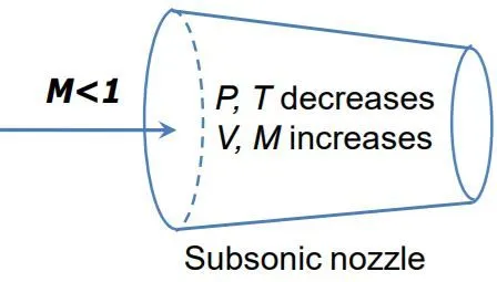
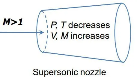
• The highest velocity that can be achievedin a converging nozzle is the sonic velocity.                                                                                                           
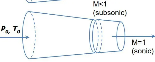
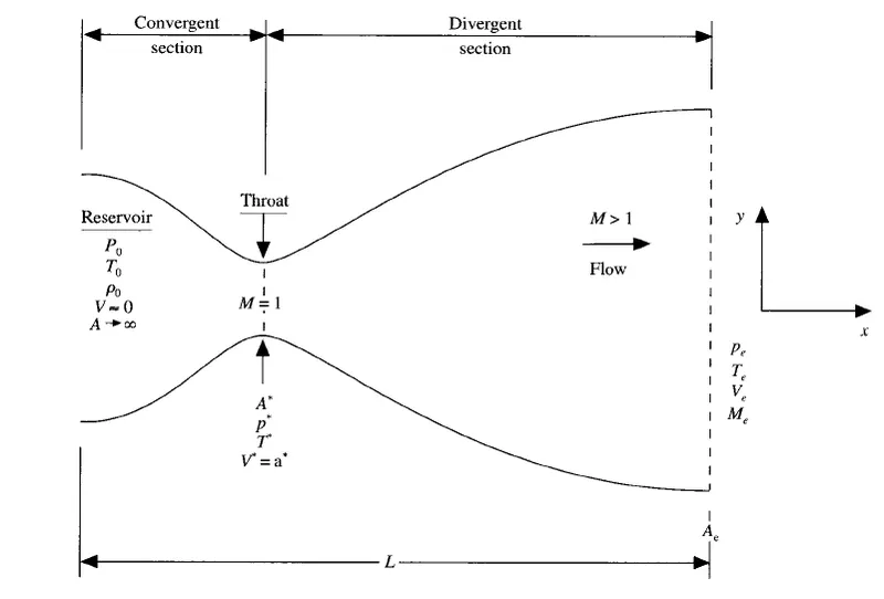
• To accelerate to supersonic velocities,diverging section after the converging section is required(Converging diverging)                                                   

CONCEPT:

1. Form Governing flow equation in PDE's,which suitable for Quasi 1D convergent-Divergent Nozzle in terms of both conservative and non-conservative forms
2. Other details like intial condition and Boundary conditions,time step calculations will be formulated.
3. Solve those PDE's using MacCormack's technique.

GOVERNING QUATIONS:

Note:Reference taken from book "Computational Fluid Dynamics"written by "JOHN D.ANDERSON"

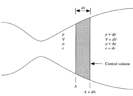
Assume Control volume(dx*1*1) in nozzle as shown below.Derive three(3) fundamental governing equations with help of Reynold's transport theorem.

`((delB)/(delt))_(sys)=(del(int_(cv)rho*b*dV))/(delt)+int_(cs)rho*b*(vecv*hatn)*dA`

Continuity Equation:

Here,b=1;dA=ds

for 1D,  `vecv*hatn=v`

`0=(del(int_(cv)rho*1*dV))/(delt)+int_(cs)rho*1*v*ds`

 Conservative form of Continuty equation:

`(del(rhoA))/(del(t))+(del(rhoAv))/(del(x))=0`

Non-Conservative form of Continuty equation:

`(del(rho))/(del(t))+rho(del(v))/(del(x))+v(del(rho))/(del(x))+rhov(del(log(A)))/(del(x))=0`

Momentum Equation:

Here,b=v;dA=ds;

for 1D,`vecv*hatn=v`

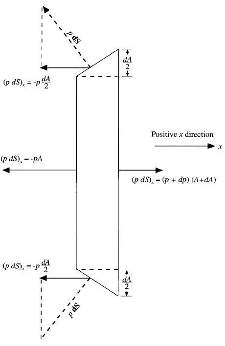
`(del(int_(cv)rho*v*dV))/(delt)+int_(cs)rho*v*v*ds=-int_(cs)(p*ds)_x`

Conservative form of Momentum equation:

`(del(rhovA))/(del(t))+(del(rhov^2A))/(del(x))=-A(del(p))/(del(x))`

Non-Conservative form of Momentum equation:

`rho(del(v))/(del(t))+rhov(del(v))/(del(x))=-(del(p))/(del(x))`

we know `p=rhoRt`

then,`(delp)/(delx)=R(rho(delT)/(delx)+T(delrho)/(delx))`

`rho(del(v))/(del(t))+rhov(del(v))/(del(x))=-R(rho(delT)/(delx)+T(delrho)/(delx))`

Energy equation:

Here,b=e+(v^2/2);dA=ds;

for 1D,`vecv*hatn=v`

`(del(int_(cv)rho*(e+(v^2/2))*dV))/(delt)+int_(cs)rho*(e+(v^2/2))*v*ds=-int_(cs)(pv)*ds`

Conservative form of Energy equation:

`(del(rhoeA))/(del(t))+(del(rhoevA))/(del(x))=-p(del(Av))/(del(x))`

Non-Conservative form of Energy equation:

`rho(del(e))/(del(t))+rhov(del(e))/(del(x))=-p(del(v))/(del(x))-pv(del(logA))/(del(x))`

we know `p=rhoRT` & `e=c_vT`

`rhoc_v(del(T))/(del(t))+rhovc_v(del(T))/(del(x))=-rhoRT((del(v))/(del(x))+v(del(logA))/(del(x)))`

But for Nozzle flow,the flow field variables are frequently expressed in terms of nondimensional variables,which are referenced to the reservoir values`(T_0,P_0,a_0;v_0)`.

Non-Dimensional variables:

Nondimensional Temperature`(T')=T/T_0`

Nondimensional density`(rho')=rho/rho_0`

Nondimensional length`(x')=x/L`

Nondimensional velocity`(v')=v/a_0`

where speed of sound at reservior`(a_0)=sqrt(gamma*r*T_0``

Nondimensional time`(t')=t/(L/a_0)`

Nondimensional area`(A')=A/(A^**)`

Substitute all nondimensional terms in governing equations.we will get Nondimensional governing equation

Dimensionless Nonconservative Form:

 For Continuity equation:

`(del(rho'))/(del(t'))+rho'(del(v'))/(del(x'))+v'(del(rho'))/(del(x'))+rho'v'(del(log(A')))/(del(x'))=0`

For Momentum equation:

`(del(v'))/(del(t'))=-v'(del(v'))/(del(x'))-1/gamma((delT')/(delx')+(T')/(rho')(delrho)/(delx))`

 For Energy equation:

`(del(T'))/(del(t'))=-v'(del(T'))/(del(x'))-(gamma-1)T'((del(v'))/(del(x'))+v'(del(logA'))/(del(x')))`

Dimensionless Conservative Form:

For Continuity equation:

`(del(rho'A'))/(del(t'))+(del(rho'A'v'))/(del(x'))=0`

For Momentum equation:

`(del(rho'v'A'))/(del(t'))+(del(rho'A'(v')^2+1/gammap'A'))/(del(x'))=1/gammap'(del(A'))/(del(x'))`

For Energy equation:

`(del(rho'((e')/(gamma-1)+gamma/2(v')^2)A'))/(del(t'))+(del(rho'((e')/(gamma-1)+gamma/2(v')^2)v'A'+p'A'v'))/(del(x'))=0`

Generic Form of Conservative form of Governing Equation:

let `u_1=rho'A'`;   `u_2=rho'A'v'`;      `u_3=rho'A'((e')/(gamma-1)+gamma/2(v')^2)`

`f_1=rho'A'v'`;      `f_2=rho'A'(v')^2+1/gammap'A'`;      `f_3=rho'((e')/(gamma-1)+gamma/2(v')^2)v'A'+p'A'v'`

`j_2=1/gammap'(delA')/(delx')`

Generic form:

`(del(u_1))/(del(t'))=-(del(f_1))/(del(x'))`

`(del(u_2))/(del(t'))=-(del(f_2))/(del(x'))+j_2`

`(del(u_3))/(del(t'))=-(del(f_3))/(del(x'))`

Hence,generic form of conservative form of governing equations are not in terms of primitive variables.It give solutions in terms of `u_1,u_2,u_3`.

From `u_1,u_2,u_3`,we can calculate primitive variables,as below:

`rho'=u_1/(A')`

`v'=u_2/u_1`

`T'=e'=(gamma-1)(u_3/u_1-gamma/2(v')^2)`

`p'=rho'T'`

Author's suggestion: for calculating `f_1,f_2,f_3,j_2`for time-marching solution

when the computer program is written with `f_1,f_2,f_3,j_2` expressed directly in terms of `rho',v',p',e'.`,instabilities develop during time-marching solutions.

So,calculate `f_1,f_2,f_3,j_2` in terms of `u_1,u_2,u_3.`

`f_1=u_2`;

`f_2=u_2^2/u_1+(gamma-1)/gamma(u_3-gamma/2u_2^2/u_1)`;

`f_3=gamma(u_2u_3)/u_1-(gamma(gamma-1))/2u_2^3/u_1^2`

`j_2=(gamma-1)/gamma(u_3-gamma/2u_2^2/u_1)(del(logA'))/(delx')`

INITIAL CONDITION & NOZZLE SHAPE:

NOZZLE SHAPE:

Nozzle ShapeA(x) is held fixed & independent of time.

`A=1+2.2(x-1.5)^2`

INITIAL CONDITION(t=0):

For Nonconservative Form:

`rho=1-0.3146x`

`T=1-0.2314x`

`v=(0.1+1.09x)T^(1/2)`

For Conservative Form:

here,Initial conditions of primitive variables are needed to calculate `u_1,u_2,u_3.`

The stability behavior of finite difference formulation using conservative form of governing equations are slightly more sensitive.So initial conditions are vary along flow direction.

`rho'=1;T'=1}0lex'le0.5`

`rho'=1-0.366(x'-0.5);T'=1-0.167(x'-0.5) }0.5lex'le1.5`

`rho'=0.634-0.3879(x'-1.5);T'=0.833-0.3507(x'-1.5) }1.5lex'le3.5`

for initial conditions only,`u_2`(local mass flow) is assumed to be constant mass flow.

`u_2=0.59`

therefore,`v'=u_2/(rho'A')`

BOUNDARY CONDITION:

Without proper implementation of boundary conditions and their numerically proper representation,we won't obtain a proper numerical solution to our flow problem

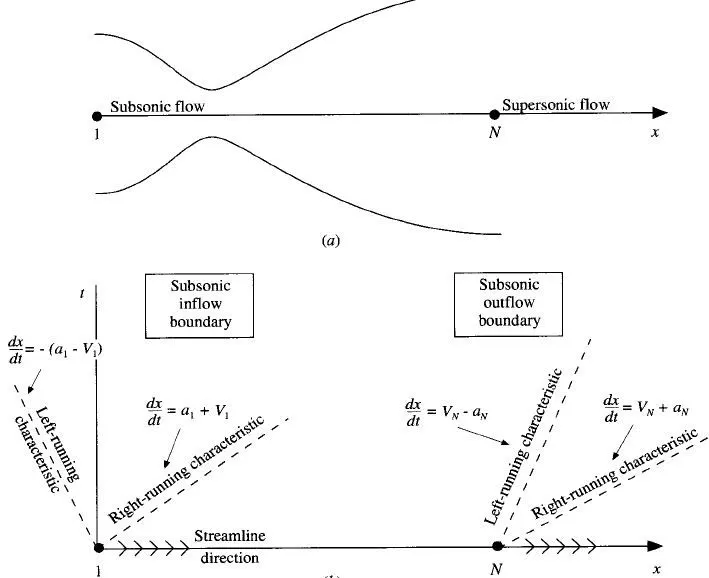
The method of characteristic tells us that at a boundary where one characteristic propagates into domain,then the value of dependent flow-field variable must be specified at that boundary, and if one characteristic line propagates out of domain,then the value of another dependent flow-field variable must be allowed to float at the boundary(it must be calculated in steps of time as a function of the timewise solution of flow field).

At point 1,left-running characteristic is propagating out of the domain,hence one variable must be float.

For Non conservative form:

`(v_1-v_2)/dx=(v_2-v_3)/dx`

`v_1=2v_2-v_3`

hence `rho=1;T=1;`}fixedindependent of time

For Conservative form:

`u_(1_(i=1))=(rho'A')_(i=1)=A'_(i=1)`

`u_(2_(i=1))=2u_(2_(i=2))-u_(2_(i=3))`

`u_3=u_1((T')/(gamma-1)+gamma/2(v')^2)`

At point N,both left running and right running characteristic is propagating out of domain.hence all variables must be float

For Non conservative form:

`v_N=2v_(N-1)-v_(N-2)`

`rho_N=2rho_(N-1)-rho_(N-2)`

`T_N=2T_(N-1)-T_(N-2)`

For conservative form:

`u_(1_(N))=2u_(1_(N-1))-u_(1_(N-2))`

`u_(2_(N))=2u_(2_(N-1))-u_(2_(N-2))`

`u_(3_(N))=2u_(3_(N-1))-u_(3_(N-2))`

TIME STEP CALCULATION:

we know,

Courant Friedrichs-Lowry criterion(cfl):

cfl=Velocity *time/grid spacing

time=cfl*(grid spacing/veocity*time)

`dt=cfl*(dx/(a+v))`

At grid point(i),

`(dt)_i^t=cfl*(dx/(a_i^t+v_i^t))`

At grid point(i+1)

`(dt)_(i+1)^t=cfl*(dx/(a_(i+1)^t+v_(i+1)^t))`

hence time step was vary from one grid point to other.

Author suggest,choose minimum value among them.

`dt=min(dt_1^t,dt_2^t,dt_3^t,dt_4^t.......dt_N^t)`

FINITE DIFFERENCE EQUATIONS:

MacCormack Method:

MacCormack method is also an explicit finite difference technique which is second-order-accurate in both space & time.

Example:MacCormack method for simple continuity equation

Predictor step:

Replace spatial derivatives on the right-handed side with forward differences.

`((delrho)/(delt))_(i)^n=-(rho_(i)^n(v_(i+1)^n-v_(i)^n)/dx+v_(i)^n(rho_(i+1)^n-rho_(i)^n)/dx)`

Solution Update:

`barrho_(i)^(n+1)=rho_(i)^n+((delrho)/(delt))_(i)^n`

Corrector step:

Substitute the predicted values into right side of continuity equation and replace the spatial derivatives with rearward differences.

`(bar(delrho)/(delt))_(i)^(n+1)=-(barrho_(i)^(n+1)(barv_(i)^(n+1)-barv_(i-1)^(n+1))/dx+barv_(i)^(n+1)(barrho_(i)^(n+1)-barrho_(i-1)^(n+1))/dx)`

`((delrho)/(delt))_(avg)=1/2(((delrho)/(delt))_(i)^(n)+(bar(delrho)/(delt))_(i)^(n+1))`

`rho_(i)^(n+1)=rho_(i)^(n)+((delrho)/(delt))_(avg)*dt`

Apply Boundary conditions

Repeat same procedure for governing equations at all time steps.

MAIN PROGRAM:

clear all
close all
clc
%%Boundary condition
%no.of grid points=N;length of nozzle=L;
N=[31,61];L=3;

for i=1:length(N)
    %non dimensional grid points=x;
x=linspace(0,L,N(i));
[dens_noncon,vel_noncon,temp_noncon,press_noncon,mach_noncon,mass_noncon,throat_area_noncon]=noncon_CDnozzle(N(i),L,i,x);
[dens_con,vel_con,temp_con,press_con,mach_con,mass_con,throat_area_con]=con_CDnozzle(N(i),L,i,x);
rho_con(i)=dens_con(701,throat_area_con);rho_noncon(i)=dens_noncon(701,throat_area_noncon);
T_noncon(i)=temp_noncon(701,throat_area_noncon);T_con(i)=temp_con(701,throat_area_con);
p_noncon(i)=press_noncon(701,throat_area_noncon);p_con(i)=press_con(701,throat_area_con);
M_noncon(i)=mach_noncon(701,throat_area_noncon);M_con(i)=mach_con(701,throat_area_con);
m_noncon(i)=mass_noncon(701,throat_area_noncon);m_con(i)=mass_con(701,throat_area_con);
if i==1
    d=13;e=15;
end
if i==2
    d=14;e=16;
end
figure(d)
plot(x,mass_con(701,:),'linewidth',1.5)
hold on
plot(x,mass_noncon(701,:),'linewidth',1.5)
hold on
plot(x,mass_con(1,:),'linewidth',1.5)
legend('conservation mass','nonconservation mass','analytical mass')
title_text=sprintf('conservative vs nonconservative vs analytical massflowrate,N=%d',N(i));
title(title_text)
figure(e)
subplot(4,1,1)
plot(x,dens_con(701,:),'*','linewidth',1.5)
hold on
plot(x,dens_noncon(701,:),'linewidth',1.5)
legend('conservative','nonconservative')
xlabel('dx')
ylabel('density')
title_text=sprintf('steady state distribution of primitive variables ,N=%d',N(i));
title(title_text)
subplot(4,1,2)
plot(x,temp_con(701,:),'*','linewidth',1.5)
hold on
plot(x,temp_noncon(701,:),'linewidth',1.5)
legend('conservative','nonconservative')
xlabel('dx')
ylabel('temperature')
subplot(4,1,3)
plot(x,press_con(701,:),'*','linewidth',1.5)
hold on
plot(x,press_noncon(701,:),'linewidth',1.5)
legend('conservative','nonconservative')
xlabel('dx')
ylabel('pressure')
subplot(4,1,4)
plot(x,mach_con(701,:),'*','linewidth',1.5)
hold on
plot(x,mach_noncon(701,:),'linewidth',1.5)
legend('conservative','nonconservative')
xlabel('dx')
ylabel('Mach number')
end
rho_noncon
rho_con
T_noncon
T_con
p_noncon
p_con
M_noncon
M_con
m_noncon
m_con

NON CONSERVATIVE MAIN PROGRAM:

function[dens,vel,temp,press,mach,mass,throat_area]=noncon_CDnozzle(N,L,i,x)
%grid spacing=dx;
dx=L/(N-1);
%non dimensional area
A=1+2.2*(x-1.5).^2;
throat_area=find(A==1);
%dimensional terms(density,temperature,velocity)
rho_dim=1-(0.3146*x);
T_dim=1-(0.2314*x);
v_dim=(0.1+(1.09*x)).*T_dim.^(0.5);
%Initial conditon
rho_initial=1;T_initial=1;gamma=1.4;R=0.718;
%c_p=1.005;c_v=0.718;R=c_p-c_v;
a_initial=(gamma*R*T_initial)^0.5;
%non dimensional terms(density,temperature,velocity)
rho=rho_dim/rho_initial;
T=T_dim/T_initial;
v=v_dim/a_initial;
p=rho.*T;
M=v./T.^0.5;
m=rho.*A.*v;
%NON-CONSERVATIVE GOVERNING EQUATION by MacCormack Technique
%Calculation of time step
cfl=0.5;
for k=1:N
   Dt(k)=cfl*(dx/((T(k)^0.5)+v(k)));
end
dt=min(Dt);
nt=1400;%no.of timestep=nt;
dens=zeros(nt,N);vel=zeros(nt,N);temp=zeros(nt,N);mass=zeros(nt,N);press=zeros(nt,N);mach=zeros(nt,N);
dens(1,:)=rho;vel(1,:)=v;temp(1,:)=T;mass(1,:)=m;press(1,:)=p;mach(1,:)=M;
for n=2:nt
dens(n,1)=rho_initial;temp(n,1)=T_initial;
[rho,v,T]= maccormack_non(N,rho,dx,v,A,T,gamma,dt);
p=rho.*T;
m=rho.*v.*A;
M=v./T.^0.5;
dens(n,:)=rho;
vel(n,:)=v;
temp(n,:)=T;
press(n,:)=p;
mach(n,:)=M;
mass(n,:)=m;
end
if i==1
    a=1;b=2;c=3;
end
if i==2
    a=7;b=8;c=9;
end

figure(a)
subplot(2,1,1)
plot(dens(:,16),'linewidth',1)
xlabel('no.of time step')
ylabel('nondimensional rho')
title_text=sprintf('non conservative,N=%d',N);
title(title_text)
grid on
subplot(2,1,2)
plot(temp(:,16),'linewidth',1)
xlabel('no.of time step')
ylabel('nondimensional Temperature')
grid on
figure(b)
subplot(2,1,1)
plot(press(:,16),'linewidth',1)
xlabel('no.of time step')
ylabel('nondimensional pressure')
title_text=sprintf('non conservative,N=%d',N);
title(title_text)
grid on
subplot(2,1,2)
plot(mach(:,16),'linewidth',1)
xlabel('no.of time step')
ylabel('nondimensional Mach')
grid on
Nt=[1,51,101,151,201];
figure(c)
plot(x,mass(Nt(1:length(Nt)),:),'linewidth',1)
hold on
plot(x,mass(701,:),'*','linewidth',1)
legend('0dt','50dt','100dt','150dt','200dt','700dt')
xlabel('dx')
ylabel('nondimensional mass flow rate')
title_text=sprintf('non conservative,N=%d',N);
title(title_text)
grid on
end

NON CONSERVATIVE ADDITIONAL PROGRAM:

function [rho,v,T]= maccormack_non(N,rho,dx,v,A,T,gamma,dt)
rho_old=rho;
v_old=v;
T_old=T;
%predictor step
for j=2:N-1
dvdx_p=(v(j+1)-v(j))/dx;
dlogAdx_p=(log(A(j+1))-log(A(j)))/dx;
drhodx_p=(rho(j+1)-rho(j))/dx;
dTdx_p=((T(j+1)-T(j))/dx);
%continuty equation
drhodt_p(j)=-1*((rho(j)*dvdx_p)+(rho(j)*v(j)*dlogAdx_p)+(v(j)*drhodx_p));
%momentum equation
dvdt_p(j)=-1*((v(j)*dvdx_p)+((1/gamma)*(dTdx_p+(T(j)/rho(j))*drhodx_p)));
%energy equation
dTdt_p(j)=-1*((v(j)*dTdx_p)+((gamma-1)*T(j)*(dvdx_p+(v(j)*dlogAdx_p))));
% solution update
rho(j)=rho(j)+(drhodt_p(j)*dt);
v(j)=v(j)+(dvdt_p(j)*dt);
T(j)=T(j)+(dTdt_p(j)*dt);
end
%corrector step
for j=2:N-1
dvdx_c=(v(j)-v(j-1))/dx;
dlogAdx_c=(log(A(j))-log(A(j-1)))/dx;
drhodx_c=(rho(j)-rho(j-1))/dx;
dTdx_c=((T(j)-T(j-1))/dx);
%continuty equation
drhodt_c(j)=-1*((rho(j)*dvdx_c)+(rho(j)*v(j)*dlogAdx_c)+(v(j)*drhodx_c));
%momentum equation
dvdt_c(j)=-1*((v(j)*dvdx_c)+((1/gamma)*(dTdx_c+(T(j)/rho(j))*drhodx_c)));
%energy equation
dTdt_c(j)=-1*((v(j)*dTdx_c)+((gamma-1)*T(j)*(dvdx_c+(v(j)*dlogAdx_c))));
end
   drhodt_avg=0.5*(drhodt_p+drhodt_c);
   dvdt_avg=0.5*(dvdt_p+dvdt_c);
   dTdt_avg=0.5*(dTdt_p+dTdt_c);
   
   for i=2:N-1
       rho(i)=rho_old(i)+(drhodt_avg(i)*dt);
       v(i)=v_old(i)+(dvdt_avg(i)*dt);
       T(i)=T_old(i)+(dTdt_avg(i)*dt);
   end
   %update inlet boundary condition
   v(1)=2*v(2)-v(3);
   %update outlet boundary condition
   rho(N)=2*rho(N-1)-rho(N-2);
   v(N)=2*v(N-1)-v(N-2);
   T(N)=2*T(N-1)-T(N-2);
   
end

CONSERVATIVE MAIN PROGRAM:

function[dens,vel,temp,press,mach,mass,throat_area]=con_CDnozzle(N,L,i,x)

%grid spacing=dx;
dx=L/(N-1);
for k=1:N
while(x(k)<=0.5)
    rho_dim(k)=1;
    T_dim(k)=1;
    break
end
while(0.5<=x(k)&&x(k)<=1.5)
   rho_dim(k)=1-(0.366*(x(k)-0.5));
   T_dim(k)=1-(0.167*(x(k)-0.5));
   break
end
while(1.5<=x(k)&&x(k)<=3.5)
   rho_dim(k)=0.634-(0.3879*(x(k)-1.5));
   T_dim(k)=0.833-(0.3507*(x(k)-1.5));
   break
end
end
%Initial conditon
rho_initial=1;T_initial=1;gamma=1.4;
%non dimensional terms
rho=rho_dim/rho_initial;
T=T_dim/T_initial;
A=1+2.2*(x-1.5).^2;
throat_area=find(A==1);
v=0.579./(rho.*A);
u1=rho.*A;
u2=rho.*A.*v;
u3=rho.*A.*((T/(gamma-1))+((gamma/2)*v.^2));
p=rho.*T;
M=v./T.^0.5;
%fixed initial condition
u1(1)=A(1);
%Calculation of time step
cfl=0.5;
for k=1:N
   Dt(k)=cfl*(dx/((T(k)^0.5)+v(k)));
end
dt=min(Dt);
nt=1400;%no.of timestep=nt;
dens=zeros(nt,N);vel=zeros(nt,N);temp=zeros(nt,N);mass=zeros(nt,N);press=zeros(nt,N);mach=zeros(nt,N);
dens(1,:)=rho;vel(1,:)=v;temp(1,:)=T;mass(1,:)=u2;press(1,:)=p;mach(1,:)=M;
%time loop
for n=2:nt
dens(n,1)=rho_initial;temp(n,1)=T_initial;
[rho,v,T,u1,u2,u3]=maccormack_con(rho,T,v,u1,u2,u3,N,dx,dt,gamma,A);
m=rho.*v.*A;
p=rho.*T;
M=v./T.^0.5;
mass(n,:)=m;
press(n,:)=p;
mach(n,:)=M;
dens(n,:)=rho;
vel(n,:)=v;
temp(n,:)=T;
end
if i==1
    a=4;b=5;c=6;
end
if i==2
    a=10;b=11;c=12;
end
figure(a)
subplot(2,1,1)
plot(dens(:,16),'linewidth',1)
xlabel('no.of time step')
ylabel('nondimensional rho')
title_text=sprintf('conservative,N=%d',N);
title(title_text)
grid on
subplot(2,1,2)
plot(temp(:,16),'linewidth',1)
xlabel('no.of time step')
ylabel('nondimensional Temperature')
grid on
figure(b)
subplot(2,1,1)
plot(press(:,16),'linewidth',1)
xlabel('no.of time step')
ylabel('nondimensional pressure')
title_text=sprintf('conservative,N=%d',N);
title(title_text)
grid on
subplot(2,1,2)
plot(mach(:,16),'linewidth',1)
xlabel('no.of time step')
ylabel('nondimensional Mach')
grid on
Nt=[1,51,101,151,201];
figure(c)
plot(x,mass(Nt(1:length(Nt)),:),'linewidth',1)
hold on
plot(x,mass(701,:),'*','linewidth',1)
legend('0dt','50dt','100dt','150dt','200dt','700dt')
xlabel('dx')
ylabel('nondimensional mass flow rate')
title_text=sprintf('conservative,N=%d',N);
title(title_text)
grid on
end

CONSERVATIVE ADDITIONAL PROGRAM:

function [rho,v,T,u1,u2,u3]=maccormack_con(rho,T,v,u1,u2,u3,N,dx,dt,gamma,A)
%rho_old=rho;T_old=T;v_old=v;
u1_old=u1;u2_old=u2;u3_old=u3;
f1=u2;
f2=(u2.^2./u1)+((gamma-1)/gamma)*(u3-(gamma/2)*(u2.^2./u1));
f3=(gamma*((u2.*u3)./u1))-((gamma*(gamma-1)/2)*(u2.^3./u1.^2));
%f1_old=f1;f2_old=f2;f3_old=f3;
%predictor step
for j=2:N-1
df1dx_p=(f1(j+1)-f1(j))/dx;
df2dx_p=(f2(j+1)-f2(j))/dx;
df3dx_p=(f3(j+1)-f3(j))/dx;
j2(j)= (1/gamma)*rho(j)*T(j)*(((A(j+1))-(A(j)))/dx);
%continuity equation
du1dt_p(j)=-1*df1dx_p;
%momentum equation
du2dt_p(j)=-1*df2dx_p+j2(j);
%energy equation
du3dt_p(j)=-1*df3dx_p;
%solution update
u1(j)=u1(j)+(du1dt_p(j)*dt);
u2(j)=u2(j)+(du2dt_p(j)*dt);
u3(j)=u3(j)+(du3dt_p(j)*dt);
rho(j)=u1(j)/A(j);
v(j)=u2(j)/u1(j);
T(j)=(gamma-1)*((u3(j)/u1(j))-((gamma/2)*(u2(j)/u1(j))^2));
end
f1=u2;
f2=(u2.^2./u1)+((gamma-1)/gamma)*(u3-(gamma/2)*(u2.^2./u1));
f3=(gamma*((u2.*u3)./u1))-((gamma*(gamma-1)/2)*(u2.^3./u1.^2));
%corrector step
for j=2:N-1
df1dx_c=(f1(j)-f1(j-1))/dx;
df2dx_c=(f2(j)-f2(j-1))/dx;
df3dx_c=(f3(j)-f3(j-1))/dx;
j2(j)=(1/gamma)*rho(j)*T(j)*((A(j)-A(j-1))/dx);
%continuity equation
du1dt_c(j)=-1*df1dx_c;
%momentum equation
du2dt_c(j)=-1*df2dx_c+j2(j);
%energy equation
du3dt_c(j)=-1*df3dx_c;
end
du1dt_avg=0.5*(du1dt_p+du1dt_c);
du2dt_avg=0.5*(du2dt_p+du2dt_c);
du3dt_avg=0.5*(du3dt_p+du3dt_c);

for i=2:N-1
   u1(i)=u1_old(i)+(du1dt_avg(i)*dt);
   u2(i)=u2_old(i)+(du2dt_avg(i)*dt);
   u3(i)=u3_old(i)+(du3dt_avg(i)*dt);
end
%update inlet boundary condition
u1(1)=A(1);
u2(1)=2*u2(2)-u2(3);
u3(1)=u1(1)*((T(1)/(gamma-1))+((gamma/2)*(u2(1)/u1(1))^2));
%update outlet boundary condition
u1(N)=2*u1(N-1)-u1(N-2);
u2(N)=2*u2(N-1)-u2(N-2);
u3(N)=2*u3(N-1)-u3(N-2);
for i=1:N
rho(i)=u1(i)/A(i);
v(i)=u2(i)/u1(i);
T(i)=(gamma-1)*((u3(i)/u1(i))-((gamma/2)*(u2(i)/u1(i))^2));
end
end

Results:

Timewise variation of primitive variables:

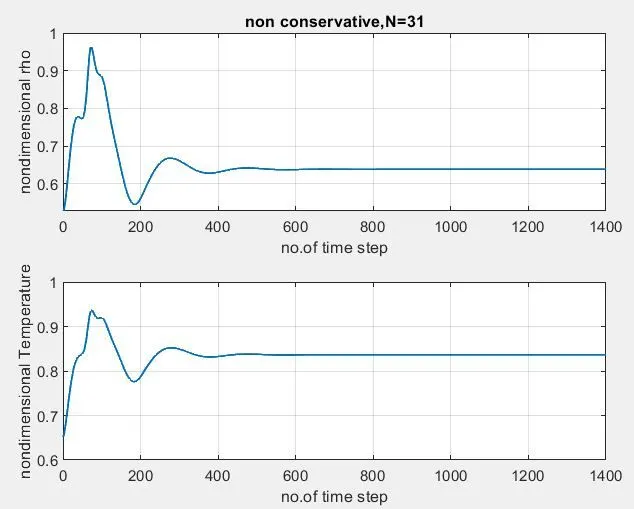
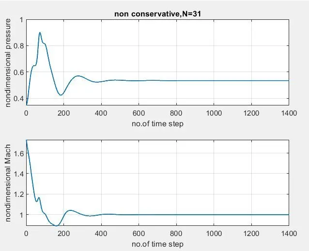
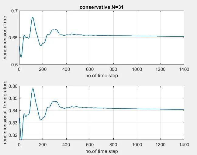
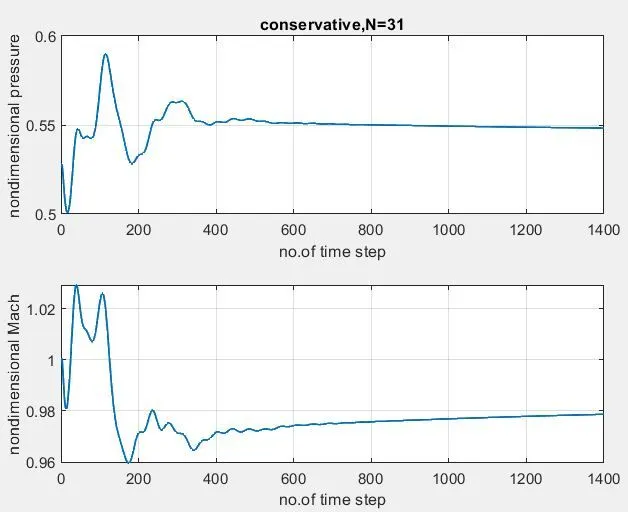
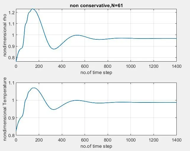
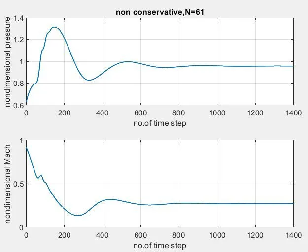
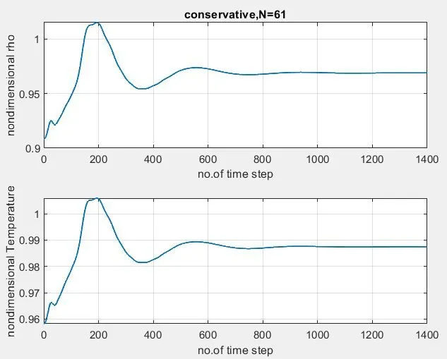
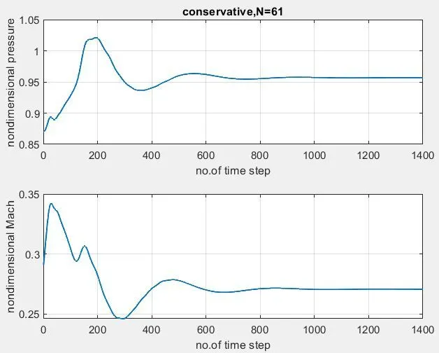
All primitive variables`(rho,p,T,M)`at grid point (i=16) plotted against different time steps

for N=31,NonConservative form

                 

for N=31,Conservative form

      

 for N=61,NonConservative form

    

for N=61,Conservative form

    

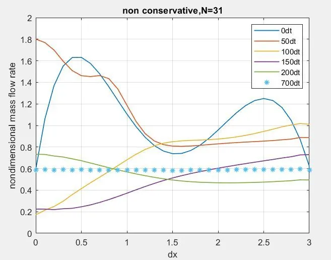
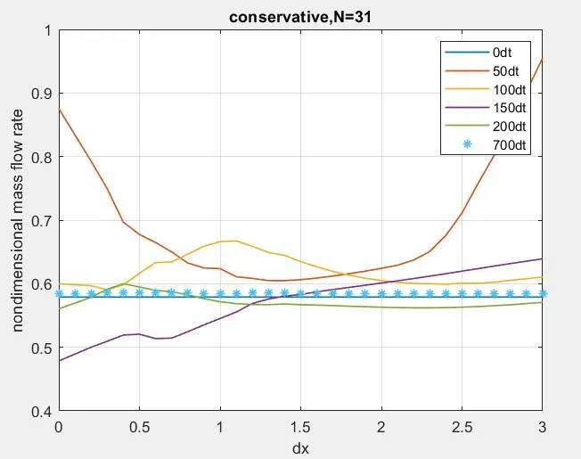
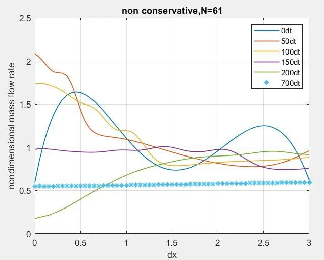
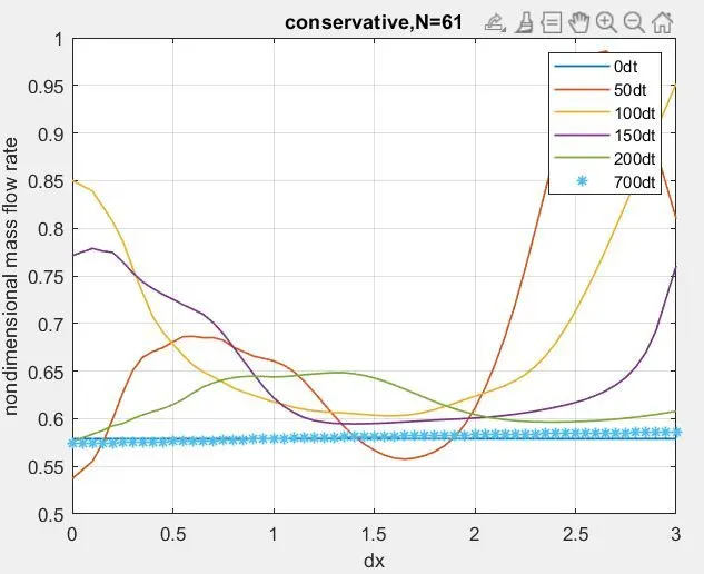
Variation of Mass flowrate distribution inside nozzle at different Timestep:

Mass flow rate at different grid points are plotted against different time steps

              

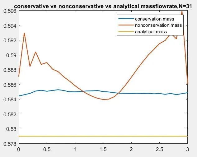
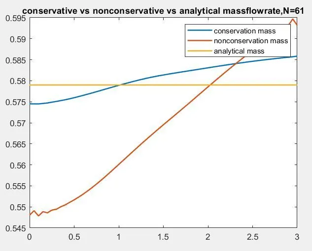
Comparison of Normalized mass flow rate distributions :

Massflow rate of both conservative and Nonconservative form at steady state(at 700th timestep) was plotted along analytical mass flow rate against different grid points.

   

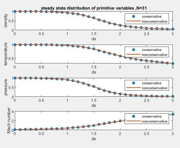
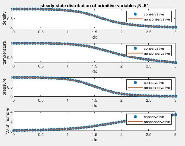
Steady-state distribution of primitive variables inside the nozzle:

Primitive variables`(rho,T,p,M)` of both conservative and Nonconservative form at steady state(at 700th timestep) was plotted against different grid points.

      

Grid Independence:

         

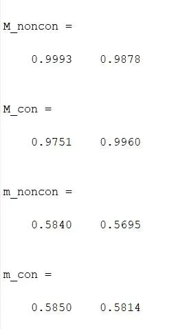
Observation:

1. After 700th time step,time wise variation of primitive variables are attain Steady state of primitive variables.
2. After 700th time step,Mass flow rate distribution at every grid point inside the nozzle become steady.
3. At 700th time step,Conservative form gives stability result,nearer to exact solution than Nonconservative form
4. At steady state,distribution of primitive variables of both conservative and Nonconservative form are similar.
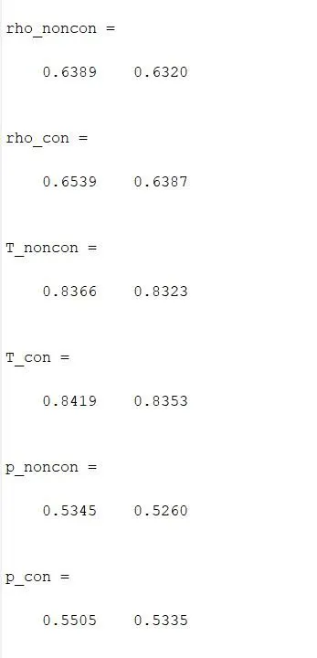
5. Obtained solution are grid independence

Primitive variables	Nonconservative form(N=31)	Nonconservative form(N=61)	Conservative form(N=31)	Conservative form(N=61)
density(`rho`)	0.6389	0.6320	0.6539	0.6387
Temperature(T)	0.8366	0.8323	0.8419	0.8353
Pressure(p)	0.5345	0.5260	0.5505	0.5335
Mach number(M)	0.9993	0.9878	0.9751	0.9960
Mass flow(m)	0.5840	0.5695	0.5850	0.5814