Week 7 - Simulation of a 1D Super-sonic nozzle flow simulation using Macormack Method
Simulation of a 1D Super-sonic nozzle flow simulation using Macormack Method
Aim :-
- Write a program to simulate the isentropic flow through a quasi 1D subsonic-supersonic nozzle.
- Derive both the conservation and non-conservation forms of the governing equation and solve them using the MacCormack’s technique.
- Write code to plot figure for steady-state distribution primitive variables inside the nozzle
- Show time wise variation of the primitive variables.
- Also, show variation of mass flow rate distribution inside the nozzle at different time step during the time-marching process.
- Compare normalized mass flow rate distribution of both forms.
- Investigate the difference between two forms of governing equation by comparing their solution.
- Lastly, perform a grid independence test on the solution and explain all experimented findings.
Objective:-
- Provide all the inputs and initial boundary condition in the main program.
- Next, firstly, write function program for conservation forms of governing equation using the MacCormack’s technique.
- Secondly, write function program for non-conservation forms of governing equation using, similar, MacCormack’s technique.
- Then call the function for specified period on time step and write code to plot steady-state distribution of primitive variables inside the nozzle inside the time step loop, for both forms.
- Next, write codes to show variation in mass flow rate distribution inside the nozzle, in the same time loop, at different time step during the time-marching process.
- Afterwards, compare normalized mass flow rate distribution of both forms by plotting results.
- Perform grid independence test to check solution is acceptable or not and explain the results.
- Finally, write detail report explaining your codes, plot and results.
McCormack method
[1] - Conservative form (Control volume is stationary)
The equations obtained from the finite control volume fixed in space, in either integral or partial differential form, are called the conservation form of the governing equation.
[2] - Non-conservative form (Control volume is moving)
The equations obtained from the finite control volume moving with fluid, in either integral or partial differential from, are called the non-conservation from of equation.
Problem Statement
Consider the steady state, isentropic flow through a converge-divergent nozzle as sketched in below figure. The flow at the inlet to the nozzle comes from a reservoir where the pressure and the temperature are denoted by `rho_0`, and `T_0`, respectively. The cross-sectional area of the reservoir is large (theoretically, `A rarr oo`), and hence the velocity is very small (`v rarr 0`), Thus, `p_0` and `T_0` are the stagnation values, or total pressure and total temperature, respectively. The flow expands isentropically to supersonic speed at the nozzle exit, where the exit pressure, temperature, velocity, and Mach number are denoted by `p_e`,`T_e`,`v_e` and `M_e`, respectively.
The flow is locally subsonic in the convergent section of the nozzle, sonic at the throat(minimum area), and supersonic at the divergent section. The sonic flow (M=1) at the throat means that the local velocity at this location is equal to the local speed of sound.
Assume that at a given section, where the cross-section area is A, the flow properties are uniform across that section. Hence, although the area of the nozzle changes as a function of distance along the nozzle, x, and therefore in reality the flow field in two dimensional. If we assume that the flow properties vary only with x; this is tantamount to assuming uniform flow properties across any given cross section. Such flow is defined as quasi-one-dimensional flow.
Following are the continuity momentum, and energy equations for the quasi one dimensional, steady state, isentropic flow.
Continuity :-
`rho_1v_1A_1 = rho_2v_2A_2`
Momentum:-
`p_1A_1+ rho_1v_1^2A_1+ int_(A_1)^(A_2) pdA = p_2A_2+ rho_2v_2^2A_2`
Energy:-
`h_1+(v_1^2)/2 = h_2 + (v_2^2)/2`
The problem setup
The governing flow equations will be couched in terms of partial differential equations suitable for the time-marching solution of quasi-one-dimensional flow
The finite-difference expressions pertaining to MacCormack's technique as applied to this problem will be set up.
Other details for the numerical solution (such as the calculation of the time step and the treatment of boundary conditions) will be formulated.
The use of the governing equations in non-conservation form
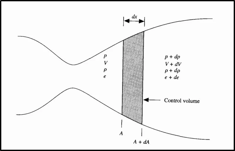
First, by referring above equations we derive it by considering small control area inside the nozzle as per shown in above figure to convert it into PDE form,
We get,
Continuity:-
`(del(rho A))/(del t) + rho A (del v)/(del x)+ rho v( del A)/(del x)+ v A (del rho)/(del x) = 0`
Momentum:-
`rho (del v)/(del t)+rho v (del v)/(del x) = -R(rho ( del T)/(del x)+T(del rho)/(del x))`
Energy:-
`rho c_v ( del T)/(del t) + rhoVc_v ( del T)/(del x) = -rhoRT [ (del v)/(del x) + v (del(ln A))/(del x)]`
Non-dimensional variable
At this stage, we could readily proceed to set up our numerical solution of above equations but these are written in terms of dimensional variable, although, this is fine, and many CFD solutions are carried out directly in terms of such dimensional variables. Indeed, this has an added engineering advantage because it gives a feeling for the magnitudes of the real physical quantities as the solution progresses. However, for nozzle flows, the flow-field variables are frequently expressed in terms of non-dimensional variables `p/p_0`, `rho/rho_0`, and `T/T_0` vary between 0 and 1, which is an “aeshetic” advantage when presenting the results. Because fluid dynamicists sealing with nozzle flows so frequently use these non-dimensional terms. Therefore by following way we will non-dimensionalize the all the entities.
Reservoir temperature and density are denoted by `T_0` and `rho_0`, respectively, we define the non-dimensional temperature and density, respectively, as
`T’ = T/(T_0) rho’ = rho/(rho_0)`
Moreover, letting L denote the length of the nozzle, we define a dimensionless length as
`x’ = x/L`
Denoting the speed of sound in the reservoir as `a_0`, where,
`a_0 = sqrt (gamma R T_0)`
We define a dimensionless velocity as
`v’ = v/(a_0)`
Also, the quantity `L/a_0` has the dimension of time, and we define a dimensionless time as
`t’ = t/(L/(a_0))`
Finally, we ratio the local area A to the sonic throat area A* and define a dimensionless area as
`A’ = A/(A**)`
After putting above value in above PDE equations we, and rearranging it properly we will get,
Continuity:-
`(del(rho’))/(del t’) = - rho’ (del v’)/(del x’)-rho’ v’( del(ln A’))/(del x’)- v’ (del rho’)/(del x’)`
Momentum:-
`(del v’)/(del t’)= - v (del v’)/(del x’) - 1/gamma ( ( del T’)/(del x’)+(T’)/(rho’)(del rho’)/(del x’))`
Energy:-
`( del T’)/(del t’) = -v’ ( del T’)/(del x’) -(gamma-1)T’ [ (del v’)/(del x’) + v '[(del(ln A’))/(del x’)]`
Mac-Cormack’s technique
Now we can proceed to the next part, namely, the setting up of the finite-difference expression using Mac-Cormack’s explicit technique for the numerical solution. To implement a finite-difference solution, we divide the x axis along the nozzle into a number of discrete grid points , as sown in below figure.
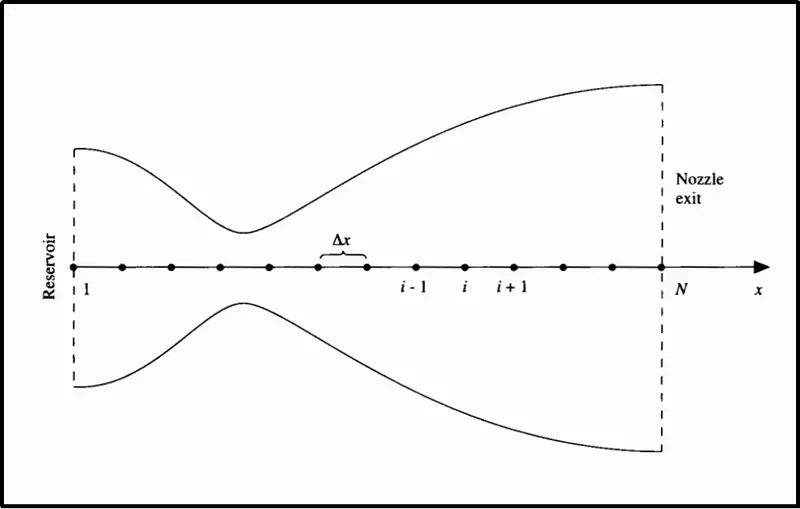
The first grid point labeled point 1, is assumed to be in the reservoir.The points are evenly distributed along the x axis, with Deltax denoting the spacing between grid points. The last point, namely, that at the nozzle exit, is denoted by N; we have a total number of N grid points distributed along the axis. Point i is simply an arbitrary grid point, with points i-1 and i+1 as the adjacent points.
From here, we are going to write function program for non-conservative form.
function [rho_nc v_nc t_nc p_nc mfr_nc M_nc drhodt dvdt dtdt] = non_conservation(n,x,t_n,dx,gamma,dt_nc,rho_nc,t_nc,v_nc,a)

rho_old = rho_nc;
v_old = v_nc;
t_old = t_nc;
Predictor step
First, consider the predictor step and apply forward difference method for non-conservation form
Continuity:-
`(del(rho))/(del t)_i^t = - rho_i^t (v_(i+1)^t-v_i^t)/(Delta x)-rho_i^t v_i^t( ln A_(i+1)-ln A_i)/(Delta x)- v_i^t ( rho_(i+1)^t-rho_i^t)/(Delta x)`
Momentum:-
`(del v)/(del t)_i^t= - v_i^t (v_(i+1)^t-v_i^t)/(Delta x) - 1/gamma ( (T_(i+1)^t-T_i^t)/(Delta x)+T_i^t/rho_i^t (rho_(i+1)^t-rho_i^t)/(Delta x))`
Energy:-
`( del T)/(del t) _i^t= -v_i^t (T_(i+1)^t - T_i^t)/(Delta x) -(gamma-1)T_i^t [ (v_(i+1)^t- v_i^t)/(Deltax) + v_i^t (( ln A_(i+1)-ln A_i)/(Delta x))]`
%% Predictor method
for j = 2:n-1

    dvdx = (v_nc(j+1)-v_nc(j))/dx;
    drhodx = (rho_nc(j+1)-rho_nc(j))/dx;
    dtdx = (t_nc(j+1)-t_nc(j))/dx;
dlogadx = (log(a(j+1))-log(a(j)))/dx;


    % Continuty Equation
    drhodt_p(j) = -rho_nc(j)*dvdx-rho_nc(j)*v_nc(j)*dlogadx - v_nc(j)*drhodx;


    % Momentum Equation
    dvdt_p(j) = -v_nc(j)*dvdx-(1/gamma)*(dtdx + (t_nc(j)/rho_nc(j))*drhodx);


    % Energy Equation
    dtdt_p(j) = -v_nc(j)*dtdx - ((gamma-1)*t_nc(j))*(dvdx + v_nc(j)*dlogadx);
We obtain predicted values of rho, v, and T denoted by barred quantities, from
`bar rho_i^(-t+Deltat) = rho_i^t + ((del rho)/(del t)_i^t) Delta t`
`bar v_i^(-t+Deltat) = v_i^t + ((del v)/(del t)_i^t )Delta t`
`bar T_i^(-t+Deltat) = T_i^t + ((del T)/(del t)_i^t )Delta t`
    %% solution update
    rho_nc(j) = rho_nc(j) + drhodt_p(j)*dt_nc;
    v_nc(j) = v_nc(j) + dvdt_p(j)*dt_nc;
    t_nc(j) = t_nc(j) + dtdt_p(j)*dt_nc;
`rho_i^t`, `v_i^t`, and `T_i^t` are known values at time `t`.
Corrected step
Moving to the corrected step, we return to previous equations replace the spatial derivatives with rearward differences, using the predicted quantities.
Continuity:-
`bar((del(rho))/(del t))_i^(t+Deltat) = - rho_i^(t+Deltat) (V_i^(t+Deltat)-V_(i-1)^(t+Deltat))/(Delta x)-rho_i^(t+Deltat) V_i^(t+Deltat) (( ln A_i-ln A_(i-1))/(Delta x)- V_i^(t+Deltat)( rho_i^(t+Deltat) -rho_(i-1)^(t+Deltat))/(Delta x) )`
Momentum:-
`bar((del v)/(del t))_i^(t+Deltat)= - V_i^(t+Deltat)( (V_(i+1)^t-V_(I-1)^-t+Deltat))/(Delta x) - 1/gamma ( (T_i^(-t+Deltat)-T_(i-1)^(t+Deltat))/(Delta x)+T_i^(t+Deltat)/rho_i^(t+Deltat) (rho_(i+1)^t-rho_(i-1)^(t+Deltat))/(Delta x))`
Energy:-
`bar(( del T)/(del t))_i^(t+Deltat)= -V_i^(-t+Deltat) (T_i^(t+Deltat) - T_(i-1)^(t+Deltat))/(Delta x) -(gamma-1)T_i^(t+Deltat) [ (V_i^(t+Deltat)- V_(i-1)^(t+Deltat))/(Deltax) +V_i^(t+Deltat) [( ln A_i-ln A_(i-1))/(Delta x)]`
%% Corrector method
for j = 2:n-1
    dvdx = (v_nc(j)-v_nc(j-1))/dx;
    drhodx = (rho_nc(j)-rho_nc(j-1))/dx;
    dtdx = (t_nc(j)-t_nc(j-1))/dx;
    dlogadx = (log(a(j))-log(a(j-1)))/dx;


    % Continuty equation
    drhodt_c(j) = -rho_nc(j)*dvdx -rho_nc(j)*v_nc(j)*dlogadx - v_nc(j)*drhodx;

    % Momentum equation
    dvdt_c(j) = -v_nc(j)*dvdx -(1/gamma)*(dtdx + (t_nc(j)/rho_nc(j))*drhodx);

    % Energy Equation
    dtdt_c(j) = -v_nc(j)*dtdx -(gamma-1)*t_nc(j)*(dvdx + v_nc(j)*dlogadx);

end
Next, calculate the average time derivative
`(del(rho))/(del t)_(av) = 0.5[((del(rho))/(del t))_i^t +bar((del(rho))/(del t))_i^(t+Deltat) ]`
`(del V)/(del t)_(aV)= 0.5[((del V)/(del t))_i^t +bar((del V)/(del t))_i^(t+Deltat) ]`
`( del T)/(del t)_(av)=0.5[(( del T)/(del t))_i^t +bar(( del T)/(del t))_i^(t+Deltat) ]`
% Compute the average time derivative
drhodt = 0.5*(drhodt_p + drhodt_c);
dvdt = 0.5*(dvdt_p + dvdt_c);
dtdt = 0.5*(dtdt_p + dtdt_c);
Finally, we have the corrected values of the flow-field variables at time t+Delta t
`rho_i^(t+Delta t) = rho_i^t + ((del rho)/(del t))_aV Delta t`
`v_i^(t+Delta t) = v_i^t + ((del v)/(del t))_aV Delta t`
`T_i^(t+Delta t) = T_i^t + ((del T)/(del t))_aV Delta t`
%% final solution Update
for i = 2:n-1
    rho_nc(i) = rho_old(i) + drhodt(i)*dt_nc;
    v_nc(i) = v_old(i) + dvdt(i)*dt_nc;
    t_nc(i) = t_old(i) + dtdt(i)*dt_nc;
end
Boundary condition
Inflow boundary condition.
`V_1 = 2V_2 - V_3`
Outflow boundary condition
`V_N = 2V_(N-1)-V_(N-2)`
`rho_N = 2rho_(N-1)-rho_(N-2)`
`p_N = 2p_(N-1)- p_(N-2)`
%% Apply the boundary conditions
% Inlet
v_nc(1) = 2*v_nc(2) - v_nc(3);

% Outlet
v_nc(n) = 2*v_nc(n-1) - v_nc(n-2);
rho_nc(n) = 2*rho_nc(n-1) - rho_nc(n-2);
t_nc(n) = 2*t_nc(n-1) - t_nc(n-2);
Calculate pressure, mass flow rate and mach number
% Pressure
p_nc = rho_nc.*t_nc;

% Mass Flow rate
mfr_nc = rho_nc.*a.*v_nc;

% Mach Number
M_nc = v_nc./(t_nc.^0.5);
The use of the governing equations in conservation form
At this stage, we know the distinction between the monconservation from and conservation form of the governing equation flow and aware of the point that, theoretically, either form of the equation is a suitable representation of the fundamental physical principles of mass conservation, Newton’s second law, and energy conservation. However, in CFD, there are some good numerical reasons to use one form or the other other for the solution of certain flow problems. An important example is the case of shock capturing, the conservation from of the equation is the proper from to employ; the nonconseravtion from will lead to poor numerical results.
In this form, we first cast the governing equation for quasi-one-dimensional flow in conservation from. Then we will set up the numerical solution of these equation using MacCormack’s technique, as applied to the subsonic-supersonic isentropic flow case.
For conservative form, we are going to start by writing function program for non-conservative form.
function [rho_c v_c t_c p_c mfr_c M_c dU1dt dU2dt dU3dt] = conservation(n,x,t_n,dx,gamma,dt_c,rho_c,t_c,v_c,a)The Basic Equations in Conservation From
These are equations for quasi-one-dimensional flow. They are already in conservation form.
Continuity:-
`(del(rho A))/(del t) + (del(rho Av)/(del x))=0`
Momentum:-
`(del(rho A v))/(del t) + (del(rho Av^2)/(del x))=-A(del p)/(del x)`
Energy:-
`(del[rho(e+v^2/2)A])/(del t) + (del[rho(e+v^2/2)Av])/(del x) = 0`
Nondimensionalizing the above equation variable as we did in previous non-conservation form
Continuity:-
`(del(rho’ A’))/(del t’) + (del(rho’ A’V’)/(del x’))=0`
Momentum:-
`(del(rho’ A’ V’))/(del t’) + (del[rho’ A’V’^2+(1/gamma)p’A’])/(del x’)=1/gamma p’(del A’)/(del x’)`
Let us define non-dimensional internal energy as follows:
`e’=e/(e_0)` where `e_0=c_v T_0 = (RT_0)/(gamma-1)`
Energy:-
`(del[rho’((e’)/(gamma-1)+gamma/2V’^2)A’])/(del t’) + (del[rho’((e’)/(gamma-1)+gamma/2V^2)A’V’+p’A’V’])/(del x) = 0`
Above equations are the nondimensional conservation form of the continuity, momentum, and energy equations for quasi-one-dimensional flow, respectively. The equation for quasi-one-dimensional flow can be expressed in a generic form. Let us define the elements of the solution vectors U, and the Flux vector F, and the source term J as follows.
`U_1 = rho’ A’`
`U_2 = rho’ A’V’`
`U_3 = rho’((e’)/(gamma-1)+gamma/2 V’^2)A’`
`F_1 = rho’ A’V’`
`F_2 = rho’ A’V’^2 + 1/gamma p’ A’`
`F_3 = rho’((e’)/(gamma-1)+gamma/2 V’^2)V’A’+p’A’V’`
`J_2 = 1/gamma p’ (rhoA’)/(rhox’)`
Pure form of flux term
`F_1 = U_2`
`F_2 = (U_2^2)/(U_1)+(gamma-1)/gamma(U_3-gamma/2 (U_2^2)/(U_1))`
`F_3 = gamma (U_2 U_3)/U_1 - (gamma(gamma-1))/2 (U_2^3)/(U_1^2)`
`J_2 = (gamma-1)/gamma (U_3-gamma/2 (U_2^2)/(U_1))(del(ln A’))/(del x’)`
% solution terms
U1 = rho_c.*a;
U2 = rho_c.*a.*v_c;
U3 = U1.*((t_c/(gamma-1))+(gamma/2).*(v_c.^2));

U1_old = U1;
U2_old = U2;
U3_old = U3;

%% Predictor method
for j = 2:n-1

    F1 = U2;
    F2 = ((U2.^2)./U1)+(((gamma-1)/gamma)*(U3-((gamma/2)*((U2.^2)./U1))));
    F3 = ((gamma*U2.*U3)./U1)-(gamma*(gamma-1)*(U2.^3))./(2*U1.^2);
Using this element above equations can be written
`(delU_1)/(del t,)=-(delF_1)/(del x,)`
`(delU_2)/(del t,)=-(delF_2)/(del x,) + J_2`
`(delU_3)/(del t,)=-(delF_3)/(del x,)`
And these are the governing equations for quasi-one-dimensional flow
We are going to descritize the equation using forward difference method for predictor step.
    %% Predictor
    % Continuty Equation
    dU1dt_p(j) = -((F1(j+1)-F1(j))/dx);

    % Momentum Equation
    dU2dt_p(j) = -((F2(j+1)-F2(j))/dx)+j2(j);

    % Energy Equation
    dU3dt_p(j) = -((F3(j+1)-F3(j))/dx);
Same way as we did in non- conservative form, we are going to update the solution.
    %% solution update
    U1(j) = U1(j) + dU1dt_p(j)*dt_c;
    U2(j) = U2(j) + dU2dt_p(j)*dt_c;
    U3(j) = U3(j) + dU3dt_p(j)*dt_c;
Update primitive variables. To obtain the primitive variables (`rho`,v,T,p etc), we must decode the elements `U_1`, `U_2`, and `U_3`
`rho’ = (U_1)/A’`
`v’ = (U_2)/(U_1)`
`T’ = e’ = (gamma-1)( (U_3)/(U_1)-gamma/2 v’^2)`
rho_c = U1./a;
v_c = U2./U1;
t_c = (gamma -1)*((U3./U1)-((gamma*v_c.^2)/2));
Corrected step
Update new values for corrected method
Pure form of flux term
F_1 = U_2
F_2 = (U_2^2)/(U_1)+(gamma-1)/gamma(U_3-gamma/2 (U_2^2)/(U_1))
F_3 = gamma (U_2 U_3)/U_1 - (gamma(gamma-1))/2 (U_2^3)/(U_1^2)

J_2 = (gamma-1)/gamma (U_3-gamma/2 (U_2^2)/(U_1))(del(ln A’))/(del x’)
Same as predictor step we are going to use following equation but by implementing backward difference method of deiscritization.
`(delU_1)/(del t,)=-(delF_1)/(del x,)`
`(delU_2)/(del t,)=-(delF_2)/(del x,) + J_2`
`(delU_3)/(del t,)=-(delF_3)/(del x,)`
    %% Corrector method
    % Continuty Equation
    dU1dt_c(j) = -((F1(j)-F1(j-1))/dx);

    % Momentum Equation
    dU2dt_c(j) = -((F2(j)-F2(j-1))/dx)+j2(j);

    % Energy Equation
    dU3dt_c(j) = -((F3(j)-F3(j-1))/dx);
Next, calculate the average time derivative, exactly same way we did it for the nonconservative approach.
% Compute the average time derivative
dU1dt = 0.5*(dU1dt_p + dU1dt_c);
dU2dt = 0.5*(dU2dt_p + dU2dt_c);
dU3dt = 0.5*(dU3dt_p + dU3dt_c);
Boundary condition at inlet and outlet
At inlet
`U_1 = rho’A’`
`U_2 = 2U _ (2(i=2) )- U_(2(i=3)`
`U_3 = U_1((T’)/(gamma-1)+gamma/2 v’^2)`
At outlet
`(U_1)_N = 2(U_1)_(N-1) -(U_1)_(N-2)`
`(U_2)_N = 2(U_2)_(N-1) -(U_2)_(N-2)`
`(U_3)_N = 2(U_3)_(N-1) -(U_3)_(N-2)`
%% Apply the boundary conditions
% Inlet
U1(1) = rho_c(1)*a(1);
U2(1) = 2*U2(2) - U2(3);
U3(1) = U1(1)*((t_c(1)./(gamma-1))+((gamma/2)*v_c(1).^2));

% Outlet
U1(n) = 2*U1(n-1) - U1(n-2);
U2(n) = 2*U2(n-1) - U2(n-2);
U3(n) = 2*U3(n-1) - U3(n-2);
Before setting up this numerical solution, one should know, the conservation form of equation the dependent variables (the variables for which directly obtain numbers) are not the primitive variables. To obtain the primitive variables (`rho`,v,T,p etc), we must decode the elements `U_1`, `U_2`, and `U_3`.
`rho’ = (U_1)/A’`
`v’ = (U_2)/(U_1)`
`T’ = e’ = (gamma-1)( (U_3)/(U_1)-gamma/2 v’^2)`
`p’ = rho’T’`
`e’ = e/(e_0) = (c_vT)/(c_vT_0)=T/(T_0)=T’`
`e’ = T’`
% Corrected values
rho_c = U1./a;
v_c = U2./U1;
t_c = (gamma -1)*((U3)./(U1)-(gamma/2)*(v_c.^2));

% Pressure
p_c = rho_c.*t_c;

% Mass Flow rate
mfr_c = rho_c.*a.*v_c;

% Mach Number
M_c = v_c./((t_c).^0.5);
Main Program
Now, we can start to program our main program. Firstly, as always, we will start out program with clear all, close all and clc to clear all the previous data, close all the previously opened figure window and clear all the command window respectively.
clear all       % Clear all Variables from memory
close all       % close all charts and figures
clc             % clear command window
Provide all the required input in the main program
%% Inputs
n = 31;
x = linspace(0,3,n);
dx = x(2)-x(1);
gamma = 1.4;
Nozzle shape and Initial condition
Nozzle shape
Next, we are going to provide boundary condition to the problem. Firstly, the nozzle shape, A=A(x), is specified and held fixed, independent of time. For the case illustrated in this section, we choose a parabolic area distribution given by
`A = 1 + 2.2(x-1.5)^2` `0<=x>=3`
Note that x = 1.5 is the throat of the nozzle, that the convergent section occurs for x<1.5 and that the divergent section occurs for x>1.5. This nozzle shape is drawn to scale in following figure.
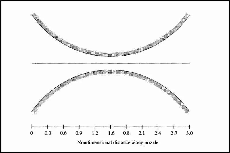
So we will put above formula in our main program.
% Area
a = 1+2.2*(x-1.5).^2;

% Throat node
t_n = find(a==1);
If we plot a we will get following results.
plot(x,a,x,-a,'linewidth',2)Result
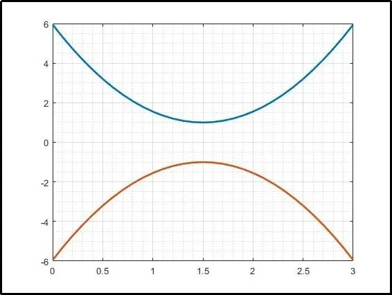
Initial conditions ( For Non-Conservation form)
To start the time marching calculation, we must stipulate initial conditions for rho, T, and v as a function of x; that is, we must set up values of rho, T, and v at time t=0
For initial condition, let us assume linear variations of the flow-field variables, as a function of x. For the present case, we assume the following values at time t=0.
`rho = 1-0.3146x`
`T = 1-0.2314x`
`V = (0.1 + 1.09)T^(1/2)`
%% Initial profile for Non-Conservative form
rho_nc = 1-0.3146*x;
t_nc = 1-0.2314*x;
v_nc = (0.1+1.09*x).*t_nc.^0.5;
Initial conditions ( For Conservation form)
For first 5 grid point we are keeping rho and T value equal to 1
`rho’ = 0.634-0.702(x’-1.5)`
`T’ = 0.833-0.4908(x’-1.5)`
For `0.5 <= x’ <= 1.5`
`rho’ = 1-0.366(x’-1.5)`
`T’ = 1-0.167(x’-1.5)`
For `1.5 <= x’ <= 3.5`
`rho’ = 0.634-0.3879(x’-1.5)`
`T’ = 0.833-0.3507(x’-1.5)`
The initial condition for the variation of v’ is synthesized bu taking advantage of the fact that one of the dependent variables in our governing equations, namely, U_2, is physically the local mass flow; that is U_2 = rho’A’v’. Therefore for the initial condition only, let us assume a constant mass flow through the nozzle and calculate v’ as
`V’= U_2/rho’A’ = 0.59/rho’A`
%% Calculate initial profile Conservative form
for i = 1:length(x)
    if x(i)<=0.5
        rho_c(i)=1;
        t_c(i)=1;
    elseif x(i)>=0.5 && x(i)<=1.5
        rho_c(i) = 1-0.366*(x(i)-0.5);
        t_c(i) = 1-0.167*(x(i)-0.5);
    elseif x(i)>=1.5 && x(i)<=3
        rho_c(i) = 0.634-0.3879*(x(i)-1.5);
        t_c(i) = 0.833-0.3507*(x(i)-1.5);
    end
end
v_c = 0.59./(rho_c.*a);
Provide time step in main program
%% No of Time step
nt = 1400;
time_range=linspace(1,nt,nt);
Calculation of time step
The governing system of equations are hyperbolic with respect to time. The stability constrain exists on this system analogous to that found, namely the Courant Number(C ).
`Delta t = C (Delta x)/(a+V)`
when the `C<= 1`, for explicit scheme, it gives the stable numerical solution. The present application to subsonic-supersonic isentropic nozzle flow is governed by nonlinear partial differential equations. In this case, the exact stability criterion for linear equation, namely, that `C<=1`, can only be viewed as general guidance for our present nonlinear problem.
Above equation is the Courant Friedrichs-Lowry (CFL) criterion for a one-dimensional flow, where V is the local flow velocity at a point in the flow and a is the local speed on sound. This equation along with `C<=1`, simply state that Delta t must be less than, or at best equal to, the time it takes a sound wave to move from one grid point to the next.
This equation is in dimensional form. However, when t,c,a, and v are nondimensionalized, the nondimensional form of above equation is exactly the same as the dimensional case. Hence, we will hereafter treat the variables in above equations as nondimensional variables defined earlier. That is, in equation, `Delta t` is the increment in nondimensional time and `Delta x` is the increment in nondimensional space; `Delta t` and `Delta x` are precisely the same as appear in the non-dimensional equations. After examine the equation, we can also note that, although `Delta x` is the same throughout the flow, both v and a are variables. Hence, at a given grid point at a given time step the equation is written as
`(Delta t)_i^t = C (Delta x)/(a_i^t+V_i^t)`
At an adjacent grid point, we have from equation
`(Delta t)_(i+1)^t = C (Delta x)/(a_(i+1)^t+V_(i+1)^t)`
the speed of sound is given by
`a = sqrtT`
% Time Step
CFL=0.5;
dt_c = min(CFL.*(dx./(sqrt(t_c)+v_c)));
dt_nc = min(CFL.*(dx./(sqrt(t_nc)+v_nc)));
Following are the analytical or exact calculation referred from the Computational fluid
Dynamics - John d. Anderson, Jr. Text Book
%% analytical calculations
a_an = a(t_n).*ones(1,nt);
rho_an = 0.634*ones(1,nt);
v_an = 0.579./(rho_an.*a_an);
t_an = 0.833*ones(1,nt);
p_an = 0.528*ones(1,nt);
% Mass flow rate for length of nt
mfr_an = 0.579*ones(1,nt);
% Mass Flow rate for length of x
mfr_an_x = 0.579*ones(1,length(x));
% Mach Number
M_an = v_an./(t_an.^0.5);
Now, at this stage we can call our function and plot the final results
Out first plot will be Steady-State Distribution of Primitive Variables along the length of nozzle for Non- Conservation form and following are the codes for that, in which we call our Non-conservative function.
tic
for k = 1:nt

    [rho_nc v_nc t_nc p_nc mfr_nc M_nc drhodt dvdt dtdt] = non_conservation(n,x,t_n,dx,gamma,dt_nc,rho_nc,t_nc,v_nc,a);


    %==============================================================================================================%
    %% Plot[1] - Plotting Steady-State Distribution of Primitive Variables for Non- Conservation form
    %           for Non- Conservation form
    %==============================================================================================================%

    figure(3);
    set(gcf, 'Position',  [10, 40, 1400, 1000])

    subplot(3,2,1)
    plot(x,rho_nc,'color','g','linewidth',1.5)
    axis([0 3 0 1.4])
    xlabel('Nozzle Length','fontweight','bold','fontsize',9)
    ylabel('Density','fontweight','bold','fontsize',9)
    heading = sprintf('Steady State Distribution of Density \nInside The Nozzle \nfor Time step = %d',k);
    title(heading,'fontsize',10);
    grid on
    grid minor

    subplot(3,2,2)
    plot(x,v_nc,'color','b','linewidth',1.5)
    axis([0 3 0 2.2])
    xlabel('Nozzle Length','fontweight','bold','fontsize',9)
    ylabel('Velocity','fontweight','bold','fontsize',9)
    heading = sprintf('Steady State Distribution of Velocity \nInside The Nozzle \nfor Time step = %d',k);
    title(heading,'fontsize',10);
    grid on
    grid minor

    subplot(3,2,3)
    plot(x,t_nc,'color','k','linewidth',1.5)
    axis([0 3 0 1.2])
    xlabel('Nozzle Length','fontweight','bold','fontsize',9)
    ylabel('Temperature','fontweight','bold','fontsize',9)
    heading = sprintf('Steady State Distribution of Temperature \nInside The Nozzle \nfor Time step = %d',k);
    title(heading,'fontsize',10);
    grid on
    grid minor

    subplot(3,2,4)
    plot(x,p_nc,'color','m','linewidth',1.5)
    axis([0 3 -0.1 1.5])
    xlabel('Nozzle Length','fontweight','bold','fontsize',9)
    ylabel('Pressure','fontweight','bold','fontsize',9)
    heading = sprintf('Steady State Distribution of Pressure \nInside The Nozzle \nfor Time step = %d',k);
    title(heading,'fontsize',10);
    grid on
    grid minor

    subplot(3,2,5)
    plot(x,mfr_nc,'color','r','linewidth',1.5)
    axis([0 3 -0.1 2.5])
    xlabel('Nozzle Length','fontweight','bold','fontsize',9)
    ylabel('Mass Flow rate','fontweight','bold','fontsize',9)
    heading = sprintf('Steady State Distribution of Mass Flow rate \nInside The Nozzle \nfor Time step = %d',k);
    title(heading,'fontsize',10);
    grid on
    grid minor

    subplot(3,2,6)
    plot(x,M_nc,'color','c','linewidth',1.5)
    axis([0 3 -0.1 4])
    xlabel('Nozzle Length','fontweight','bold','fontsize',9)
    ylabel('Mach Number','fontweight','bold','fontsize',9)
    heading = sprintf('Steady State Distribution of Mach Number \nInside The Nozzle \nfor Time step = %d',k);
    title(heading,'fontsize',10);
    grid on
    grid minor

end
Time_nc = toc
Output for the above codes(Nonconservation form)
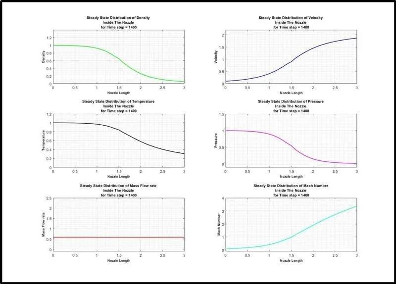
We plot same plot for the conservative form by using following codes, in which, we call our conservative function.
%% Plotting(Conservative form)
tic
for k = 1:nt

    [rho_c v_c t_c p_c mfr_c M_c dU1dt dU2dt dU3dt] = conservation(n,x,t_n,dx,gamma,dt_c,rho_c,t_c,v_c,a);


    %==============================================================================================================%
    %% Plot[2] - Plotting Steady-State Distribution of Primitive Variables for Conservation form
    %           for Conservation form
    %==============================================================================================================%

    figure(2);
    set(gcf, 'Position',  [10, 40, 1400, 1000])

    subplot(3,2,1)
    plot(x,rho_c,'color','g','linewidth',1.5)
    axis([0 3 0 1.4])
    xlabel('Nozzle Length','fontweight','bold','fontsize',9)
    ylabel('Density','fontweight','bold','fontsize',9)
    heading = sprintf('Steady State Distribution of Density \nInside The Nozzle \nfor Time step = %d',k);
    title(heading,'fontsize',10);
    grid on
    grid minor

    subplot(3,2,2)
    plot(x,v_c,'color','b','linewidth',1.5)
    axis([0 3 0 2.2])
    xlabel('Nozzle Length','fontweight','bold','fontsize',9)
    ylabel('Velocity','fontweight','bold','fontsize',9)
    heading = sprintf('Steady State Distribution of Velocity \nInside The Nozzle \nfor Time step = %d',k);
    title(heading,'fontsize',10);
    grid on
    grid minor

    subplot(3,2,3)
    plot(x,t_c,'color','k','linewidth',1.5)
    axis([0 3 0 1.2])
    xlabel('Nozzle Length','fontweight','bold','fontsize',9)
    ylabel('Temperature','fontweight','bold','fontsize',9)
    heading = sprintf('Steady State Distribution of Temperature \nInside The Nozzle \nfor Time step = %d',k);
    title(heading,'fontsize',10);
    grid on
    grid minor

    subplot(3,2,4)
    plot(x,p_c,'color','m','linewidth',1.5)
    axis([0 3 -0.1 1.5])
    xlabel('Nozzle Length','fontweight','bold','fontsize',9)
    ylabel('Pressure','fontweight','bold','fontsize',9)
    heading = sprintf('Steady State Distribution of Pressure \nInside The Nozzle \nfor Time step = %d',k);
    title(heading,'fontsize',10);
    grid on
    grid minor

    subplot(3,2,5)
    plot(x,mfr_c,'color','r','linewidth',1.5)
    axis([0 3 -0.1 2.5])
    xlabel('Nozzle Length','fontweight','bold','fontsize',9)
    ylabel('Mass Flow rate','fontweight','bold','fontsize',9)
    heading = sprintf('Steady State Distribution of Mass Flow rate \nInside The Nozzle \nfor Time step = %d',k);
    title(heading,'fontsize',10);
    grid on
    grid minor

    subplot(3,2,6)
    plot(x,M_c,'color','c','linewidth',1.5)
    axis([0 3 -0.1 4])
    xlabel('Nozzle Length','fontweight','bold','fontsize',9)
    ylabel('Mach Number','fontweight','bold','fontsize',9)
    heading = sprintf('Steady State Distribution of Mach Number \nInside The Nozzle \nfor Time step = %d',k);
    title(heading,'fontsize',10);
    grid on
    grid minor

end
Time_c = toc
Output for the above codes(Conservation form)
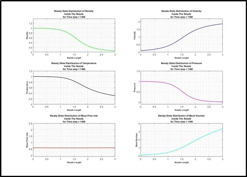
Here, we have plotted final results of all the parameters, by using both conservative and nonconservative forms, at 1400 time step.
A glimpse over both charts, conservative and nonconservative, the final results looks almost identical, which state that both methods are reliable.
Using following code we can save there video to create animation and note changes in each time step.
%% Plotting(Conservative form)
tic
for k = 1:nt

    [rho_c v_c t_c p_c mfr_c M_c dU1dt dU2dt dU3dt] = conservation(n,x,t_n,dx,gamma,dt_c,rho_c,t_c,v_c,a);


    %==============================================================================================================%
    %% Plot[2] - Plotting Steady-State Distribution of Primitive Variables for Conservation form
    %           for Conservation form
    %==============================================================================================================%

    figure(2);
    set(gcf, 'Position',  [10, 40, 1400, 1000])

    subplot(3,2,1)
    plot(x,rho_c,'color','g','linewidth',1.5)
    axis([0 3 0 1.4])
    xlabel('Nozzle Length','fontweight','bold','fontsize',9)
    ylabel('Density','fontweight','bold','fontsize',9)
    heading = sprintf('Steady State Distribution of Density \nInside The Nozzle \nfor Time step = %d',k);
    title(heading,'fontsize',10);
    grid on
    grid minor

    subplot(3,2,2)
    plot(x,v_c,'color','b','linewidth',1.5)
    axis([0 3 0 2.2])
    xlabel('Nozzle Length','fontweight','bold','fontsize',9)
    ylabel('Velocity','fontweight','bold','fontsize',9)
    heading = sprintf('Steady State Distribution of Velocity \nInside The Nozzle \nfor Time step = %d',k);
    title(heading,'fontsize',10);
    grid on
    grid minor

    subplot(3,2,3)
    plot(x,t_c,'color','k','linewidth',1.5)
    axis([0 3 0 1.2])
    xlabel('Nozzle Length','fontweight','bold','fontsize',9)
    ylabel('Temperature','fontweight','bold','fontsize',9)
    heading = sprintf('Steady State Distribution of Temperature \nInside The Nozzle \nfor Time step = %d',k);
    title(heading,'fontsize',10);
    grid on
    grid minor

    subplot(3,2,4)
    plot(x,p_c,'color','m','linewidth',1.5)
    axis([0 3 -0.1 1.5])
    xlabel('Nozzle Length','fontweight','bold','fontsize',9)
    ylabel('Pressure','fontweight','bold','fontsize',9)
    heading = sprintf('Steady State Distribution of Pressure \nInside The Nozzle \nfor Time step = %d',k);
    title(heading,'fontsize',10);
    grid on
    grid minor

    subplot(3,2,5)
    plot(x,mfr_c,'color','r','linewidth',1.5)
    axis([0 3 -0.1 2.5])
    xlabel('Nozzle Length','fontweight','bold','fontsize',9)
    ylabel('Mass Flow rate','fontweight','bold','fontsize',9)
    heading = sprintf('Steady State Distribution of Mass Flow rate \nInside The Nozzle \nfor Time step = %d',k);
    title(heading,'fontsize',10);
    grid on
    grid minor

    subplot(3,2,6)
    plot(x,M_c,'color','c','linewidth',1.5)
    axis([0 3 -0.1 4])
    xlabel('Nozzle Length','fontweight','bold','fontsize',9)
    ylabel('Mach Number','fontweight','bold','fontsize',9)
    heading = sprintf('Steady State Distribution of Mach Number \nInside The Nozzle \nfor Time step = %d',k);
    title(heading,'fontsize',10);
    grid on
    grid minor


    pause(0.001)
    M(k)= getframe(gcf);

end
Time_c = toc

% move command generates movie using frames in M array
movie(M)
% Create videofile using VideoWrite command to collect all frames in M array
videofile = VideoWriter('Conservative form.avi','Uncompressed AVI');
% open video to collet all frames from M array
open(videofile)
% writeVideo capture frames in 'M' into videofile
writeVideo(videofile,M)
% at the end close videofile
close(videofile)


%% Plotting(Non-Conservative form)
tic
for k = 1:nt

    [rho_nc v_nc t_nc p_nc mfr_nc M_nc drhodt dvdt dtdt] = non_conservation(n,x,t_n,dx,gamma,dt_nc,rho_nc,t_nc,v_nc,a);


    %==============================================================================================================%
    %% Plot[1] - Plotting Steady-State Distribution of Primitive Variables for Non- Conservation form
    %           for Non- Conservation form
    %==============================================================================================================%

    figure(1);
    set(gcf, 'Position',  [10, 40, 1400, 1000])

    subplot(3,2,1)
    plot(x,rho_nc,'color','g','linewidth',1.5)
    axis([0 3 0 1.4])
    xlabel('Nozzle Length','fontweight','bold','fontsize',9)
    ylabel('Density','fontweight','bold','fontsize',9)
    heading = sprintf('Steady State Distribution of Density \nInside The Nozzle \nfor Time step = %d',k);
    title(heading,'fontsize',10);
    grid on
    grid minor

    subplot(3,2,2)
    plot(x,v_nc,'color','b','linewidth',1.5)
    axis([0 3 0 2.2])
    xlabel('Nozzle Length','fontweight','bold','fontsize',9)
    ylabel('Velocity','fontweight','bold','fontsize',9)
    heading = sprintf('Steady State Distribution of Velocity \nInside The Nozzle \nfor Time step = %d',k);
    title(heading,'fontsize',10);
    grid on
    grid minor

    subplot(3,2,3)
    plot(x,t_nc,'color','k','linewidth',1.5)
    axis([0 3 0 1.2])
    xlabel('Nozzle Length','fontweight','bold','fontsize',9)
    ylabel('Temperature','fontweight','bold','fontsize',9)
    heading = sprintf('Steady State Distribution of Temperature \nInside The Nozzle \nfor Time step = %d',k);
    title(heading,'fontsize',10);
    grid on
    grid minor

    subplot(3,2,4)
    plot(x,p_nc,'color','m','linewidth',1.5)
    axis([0 3 -0.1 1.5])
    xlabel('Nozzle Length','fontweight','bold','fontsize',9)
    ylabel('Pressure','fontweight','bold','fontsize',9)
    heading = sprintf('Steady State Distribution of Pressure \nInside The Nozzle \nfor Time step = %d',k);
    title(heading,'fontsize',10);
    grid on
    grid minor

    subplot(3,2,5)
    plot(x,mfr_nc,'color','r','linewidth',1.5)
    axis([0 3 -0.1 2.5])
    xlabel('Nozzle Length','fontweight','bold','fontsize',9)
    ylabel('Mass Flow rate','fontweight','bold','fontsize',9)
    heading = sprintf('Steady State Distribution of Mass Flow rate \nInside The Nozzle \nfor Time step = %d',k);
    title(heading,'fontsize',10);
    grid on
    grid minor

    subplot(3,2,6)
    plot(x,M_nc,'color','c','linewidth',1.5)
    axis([0 3 -0.1 4])
    xlabel('Nozzle Length','fontweight','bold','fontsize',9)
    ylabel('Mach Number','fontweight','bold','fontsize',9)
    heading = sprintf('Steady State Distribution of Mach Number \nInside The Nozzle \nfor Time step = %d',k);
    title(heading,'fontsize',10);
    grid on
    grid minor


    pause(0.001)
    N(k)= getframe(gcf);

end
Time_c = toc

% move command generates movie using frames in N array
movie(N)
% Create videofile using VideoWrite command to collect all frames in N array
videofile = VideoWriter('Non-Conservative form.avi','Uncompressed AVI');
% open video to collet all frames from N array
open(videofile)
% writeVideo capture frames in 'N' into videofile
writeVideo(videofile,N)
% at the end close videofile
close(videofile)
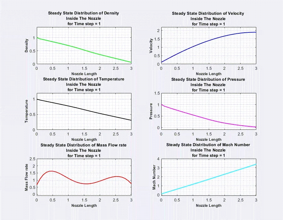
Output for above codes
[A] Nonconservation form
[B] Conservation form
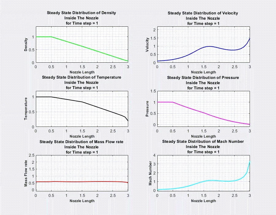
In above gif we can see, how both, conservative and nonconservative form, converge the results with each time step. and one thing we can notice is that, in nonconservation form, at the early time steps, primitive vary its value in volatile way than the conservation form, which make sense as it is implement to reduce shock waves generated in range of values of the parameters.
Time-wise variation of the Primitive variables
Next codes are to plot time wise variation of primitive variables. We will calculate this primitives value at nozzle throat area so we have to extract the values of all parameters at nozzle throat node.
%% Plotting(Non-Conservative form)
tic
for k = 1:nt

    [rho_nc v_nc t_nc p_nc mfr_nc M_nc drhodt dvdt dtdt] = non_conservation(n,x,t_n,dx,gamma,dt_nc,rho_nc,t_nc,v_nc,a);

    %% Throat Values
    rho_nc_throat(k) = rho_nc(t_n);
    v_nc_throat(k) = v_nc(t_n);
    t_nc_throat(k) = t_nc(t_n);
    p_nc_throat(k) = p_nc(t_n);
    mfr_nc_throat(k) = mfr_nc(t_n);
    M_nc_throat(k) = M_nc(t_n);
end
Time_nc = toc


%% Plotting(Conservative form)
tic
for k = 1:nt

    [rho_c v_c t_c p_c mfr_c M_c dU1dt dU2dt dU3dt] = conservation(n,x,t_n,dx,gamma,dt_c,rho_c,t_c,v_c,a);


    %% Throat Values
    rho_c_throat(k) = rho_c(t_n);
    v_c_throat(k) = v_c(t_n);
    t_c_throat(k) = t_c(t_n);
    p_c_throat(k) = p_c(t_n);
    mfr_c_throat(k) = mfr_c(t_n);
    M_c_throat(k) = M_c(t_n);
end
Time_c = toc


%==============================================================================================================%
%% Plot[6] - Timewise variations of the density, temperature, pressure, and Mach number at the nozzle throat
%==============================================================================================================%

figure(6);
set(gcf, 'Position',  [10, 40, 1400, 1000])

subplot(3,2,1)
plot(time_range,rho_c_throat,'color','b','linewidth',1.5)
hold on
plot(time_range,rho_nc_throat,'color','g','linewidth',1.5)
plot(time_range,rho_an,'color','k','linewidth',1.5)
legend({'Conservation form','Non-Conservation form','Exact '},'fontweight','bold','fontsize',8)
xlabel('Number of time steps','fontweight','bold','fontsize',9)
ylabel('Density','fontweight','bold','fontsize',9)
heading = sprintf('Timewise variations of the Density \nat the nozzle throat');
title(heading,'fontsize',10);
grid on
grid minor

subplot(3,2,2)
plot(time_range,v_c_throat,'color','b','linewidth',1.5)
hold on
plot(time_range,v_nc_throat,'color','g','linewidth',1.5)
plot(time_range,v_an,'color','k','linewidth',1.5)
legend({'Conservation form','Non-Conservation form','Exact '},'fontweight','bold','fontsize',8)
xlabel('Number of time steps','fontweight','bold','fontsize',9)
ylabel('Velocity','fontweight','bold','fontsize',9)
heading = sprintf('Timewise variations of the Velocity \nat the nozzle throat');
title(heading,'fontsize',10);
grid on
grid minor

subplot(3,2,3)
plot(time_range,t_c_throat,'color','b','linewidth',1.5)
hold on
plot(time_range,t_nc_throat,'color','g','linewidth',1.5)
plot(time_range,t_an,'color','k','linewidth',1.5)
legend({'Conservation form','Non-Conservation form','Exact '},'fontweight','bold','fontsize',8)
xlabel('Number of time steps','fontweight','bold','fontsize',9)
ylabel('Temperature','fontweight','bold','fontsize',9)
heading = sprintf('Timewise variations of the Temperature \nat the nozzle throat');
title(heading,'fontsize',10);
grid on
grid minor

subplot(3,2,4)
plot(time_range,p_c_throat,'color','b','linewidth',1.5)
hold on
plot(time_range,p_nc_throat,'color','g','linewidth',1.5)
plot(time_range,p_an,'color','k','linewidth',1.5)
legend({'Conservation form','Non-Conservation form','Exact '},'fontweight','bold','fontsize',8)
xlabel('Number of time steps','fontweight','bold','fontsize',9)
ylabel('Pressure','fontweight','bold','fontsize',9)
heading = sprintf('Timewise variations of the Pressure \nat the nozzle throat');
title(heading,'fontsize',10);
grid on
grid minor

subplot(3,2,5)
plot(time_range,mfr_c_throat,'color','b','linewidth',1.5)
hold on
plot(time_range,mfr_nc_throat,'color','g','linewidth',1.5)
plot(time_range,mfr_an,'color','k','linewidth',1.5)
legend({'Conservation form','Non-Conservation form','Exact '},'fontweight','bold','fontsize',8)
xlabel('Number of time steps','fontweight','bold','fontsize',9)
ylabel('Mass Flow rate','fontweight','bold','fontsize',9)
heading = sprintf('Timewise variations of the Mass Flow rate \nat the nozzle throat');
title(heading,'fontsize',10);
grid on
grid minor

subplot(3,2,6)
plot(time_range,M_c_throat,'color','b','linewidth',1.5)
hold on
plot(time_range,M_nc_throat,'color','g','linewidth',1.5)
plot(time_range,M_an,'color','k','linewidth',1.5)
legend({'Conservation form','Non-Conservation form','Exact '},'fontweight','bold','fontsize',8)
xlabel('Number of time steps','fontweight','bold','fontsize',9)
ylabel('Mach Number','fontweight','bold','fontsize',9)
heading = sprintf('Timewise variations of the Mach Number \nat the nozzle throat');
title(heading,'fontsize',10);
grid on
grid minor
Output for above codes
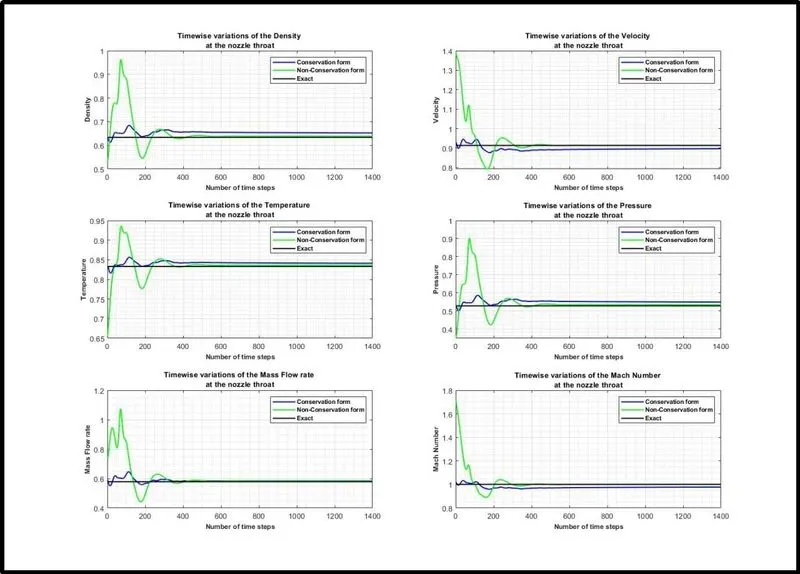
The graph exhibits the results of time- wise variation of primitives at the nozzle throat, in which, in the approach toward the steady-state solution, at larger values of time( after large number of time steps), the changes in the flow field variables from one time step to the next become smallet and approach zero in the limit of large time. At this stage, the steady state has been achieved, and the calculation can be stopped.
The largest changes occurring in each parameter at early times, after which the final, steady-state value is approached almost asymptotically.
If we compare between conservation and nonconservation form, the changes occur in nonconservation in early time step is far higher than the conservative form.
And accuracy of the final results in all other parameters, except mass flow rate, is lower with the conservative form.
Residual plot - changes in residual with respect to time step.
It is interesting to examine the variation of the time derivatives as a function of time itself, or equivalently as a function of the number of time steps. Once again focusing on the nozzle throat (at grid point i=16). As example, below figure gives the variation of the time derivation of nondimensional density and velocity as a function of the number of time step.
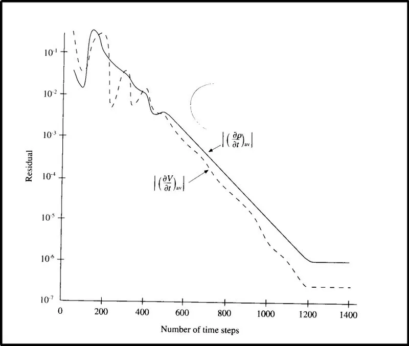
These are the average time derivatives calculated from following equations.
`(del(rho))/(del t)_(av) = 0.5[((del(rho))/(del t))_i^t +bar((del(rho))/(del t))_i^(t+Deltat) ]`
`(del v)/(del t)_(av)= 0.5[((del v)/(del t))_i^t +bar((del v)/(del t))_i^(t+Deltat) ]`
`( del T)/(del t)_(av)=0.5[(( del T)/(del t))_i^t +bar(( del T)/(del t))_i^(t+Deltat) ]`
We might visualize that what is being plotted in above figure are the numerical values of the right-hand side of these equations. As time progresses and as the steady-state is approached, the right-hand side of these equations should approach zero. Since the numerical values of the right-hand side are not precisely zero, they are called residuals.
Therefor, in coding we will get 31 residual value for each time step of every time derivative so we will select maximum residual value for our plot. Hence, following way we will write our codes.
%% Plotting(Non-Conservative form)
tic
for k = 1:nt

    [rho_nc v_nc t_nc p_nc mfr_nc M_nc drhodt dvdt dtdt] = non_conservation(n,x,t_n,dx,gamma,dt_nc,rho_nc,t_nc,v_nc,a);


    %% Residuals
    residuals_1_nc(k) = max(abs(drhodt));
    residuals_2_nc(k) = max(abs(dvdt));
    residuals_3_nc(k) = max(abs(dtdt));


    %% Throat Values
    rho_nc_throat(k) = rho_nc(t_n);
    v_nc_throat(k) = v_nc(t_n);
    t_nc_throat(k) = t_nc(t_n);
    p_nc_throat(k) = p_nc(t_n);
    mfr_nc_throat(k) = mfr_nc(t_n);
    M_nc_throat(k) = M_nc(t_n);
end
Time_nc = toc


%% Plotting(Conservative form)
tic
for k = 1:nt

    [rho_c v_c t_c p_c mfr_c M_c dU1dt dU2dt dU3dt] = conservation(n,x,t_n,dx,gamma,dt_c,rho_c,t_c,v_c,a);


    %% Residuals
    residuals_1_c(k) = max(abs(dU1dt));
    residuals_2_c(k) = max(abs(dU2dt));
    residuals_3_c(k) = max(abs(dU3dt));


    %% Throat Values
    rho_c_throat(k) = rho_c(t_n);
    v_c_throat(k) = v_c(t_n);
    t_c_throat(k) = t_c(t_n);
    p_c_throat(k) = p_c(t_n);
    mfr_c_throat(k) = mfr_c(t_n);
    M_c_throat(k) = M_c(t_n);
end
Time_c = toc


%==============================================================================================================%
%% Plot[7] - Timewise variations in residual
%==============================================================================================================%

figure(7)
subplot(1,2,1)
set(gcf, 'Position',  [10, 40, 1400, 900])
plot(time_range,residuals_1_c,'color','r','linewidth',1.5)
hold on
plot(time_range,residuals_2_c,'color','b','linewidth',1.5)
plot(time_range,residuals_3_c,'color','g','linewidth',1.5)
xlabel('Number of time steps','fontweight','bold','fontsize',12)
ylabel('Residual','fontweight','bold','fontsize',12)
legend({'residual for dU_1/dt','residual for dU_2/dt','residual for dU_3/dt'},'fontweight','bold','fontsize',11)
title('Timewise variations in residual (Conservation form)','fontsize',16);
grid on
grid minor
Output for above codes
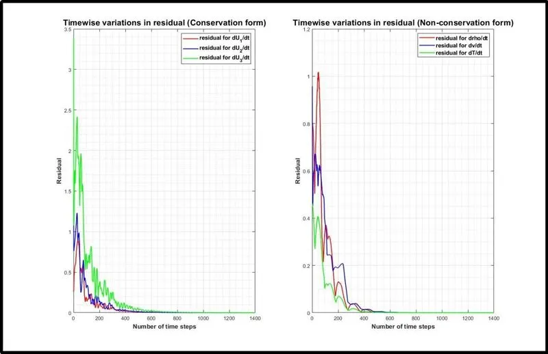
From these results, note two important aspect:-
- at early times, the time derivatives are large, and they oscillate in value. These oscillations are associated with various unsteady compression and expansion waves which propagate through the nozzle during the transient process.
- at latter times. The time derivatives rapidly grow small, charging by six orders of magnitude over a span of 1000 time steps. This is, at last, what we want to happen. In the theoretical limit of the steady state (which is achieved at infinite time), the time derivatives should go to zero. However, numerically it will never happen.
Moreover, residuals are reducing in early time steps in nonconservation method, which is after 600. On the other hand, it taking around 1000 time steps in conservation form.
Variation of mass flow rate distribution inside the nozzle at different time step during the time marching process.
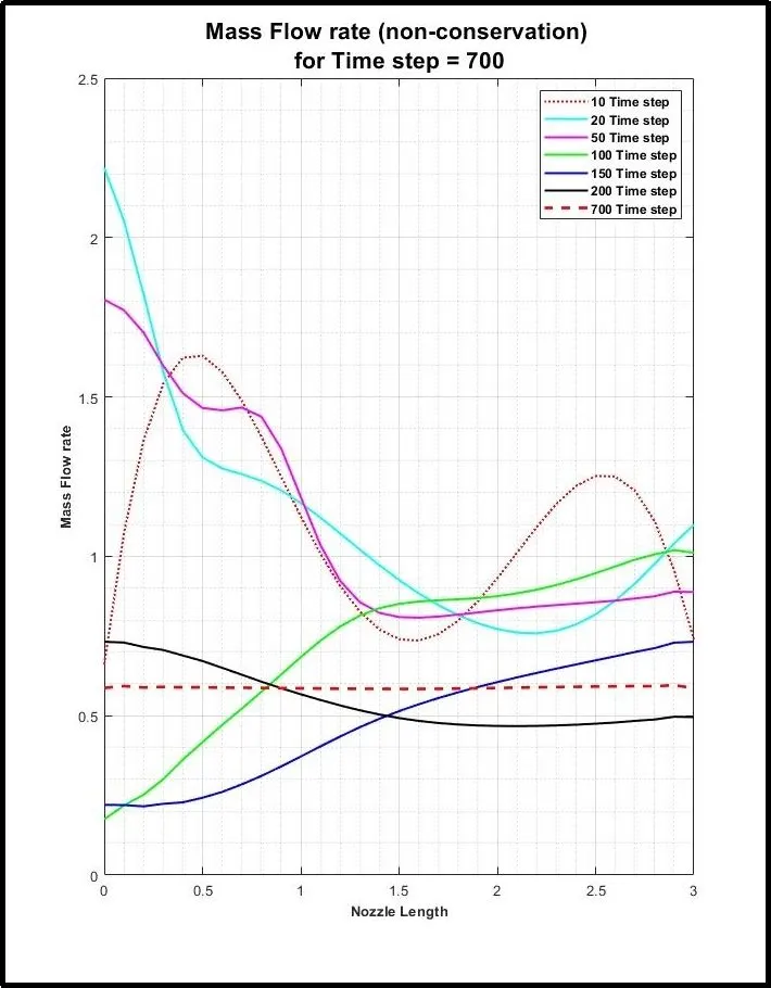
Another insight to mechanics of the time-wise variation of the flow and its approach to the steady state is provided by the mass flow rate variations.
By utilizing following code we will be able to plot variation of mass flow rate inside the nozzle plot at different time steps.
For Non-conservative form
%% Plotting(Non-Conservative form)
tic
for k = 1:nt

    [rho_nc v_nc t_nc p_nc mfr_nc M_nc drhodt dvdt dtdt] = non_conservation(n,x,t_n,dx,gamma,dt_nc,rho_nc,t_nc,v_nc,a);


    %==============================================================================================================%
    %% Plot[3] - Variation of Mass flow rate distribution inside the nozzle at different time steps
    %           for Non-conservation form
    %==============================================================================================================%

    figure(3)
    set(gcf, 'Position',  [10, 40, 700, 900])
    if k == 1
        plot(x,mfr_nc,':','color','r','linewidth',1.5)
        hold on
    elseif k == 20
        plot(x,mfr_nc,'color','c','linewidth',1.5)
    elseif k == 50
        plot(x,mfr_nc,'color','m','linewidth',1.5)
    elseif k == 100
        plot(x,mfr_nc,'color','g','linewidth',1.5)
    elseif k == 150
        plot(x,mfr_nc,'color','b','linewidth',1.5)
    elseif k == 200
        plot(x,mfr_nc,'color','k','linewidth',1.5)
    elseif k == 700
        plot(x,mfr_nc,'--','color','r','linewidth',2)
        legend({'10 Time step','20 Time step','50 Time step','100 Time step','150 Time step','200 Time step','700 Time step'},'fontweight','bold','fontsize',9)
        xlabel('Nozzle Length','fontweight','bold','fontsize',10)
        ylabel('Mass Flow rate','fontweight','bold','fontsize',10)
        heading = sprintf('Mass Flow rate (non-conservation) \nfor Time step = %d',k);
        title(heading,'fontsize',16);
        grid on
        grid minor
        hold off
    end


end
Time_nc = toc
Output of the above codes
For conservative form
%% Plotting(Conservative form)
tic
for k = 1:nt

    [rho_c v_c t_c p_c mfr_c M_c dU1dt dU2dt dU3dt] = conservation(n,x,t_n,dx,gamma,dt_c,rho_c,t_c,v_c,a);


    %==============================================================================================================%
    %% Plot[4] - Variation of Mass flow rate distribution inside the nozzle at different time steps
    %           for Conservation form
    %==============================================================================================================%

    figure(4)
    set(gcf, 'Position',  [10, 40, 700, 900])
    if k == 10
        plot(x,mfr_c,':','color','r','linewidth',1.5)
        hold on
    elseif k == 20
        plot(x,mfr_c,'color','c','linewidth',1.5)
    elseif k == 50
        plot(x,mfr_c,'color','m','linewidth',1.5)
    elseif k == 100
        plot(x,mfr_c,'color','g','linewidth',1.5)
    elseif k == 150
        plot(x,mfr_c,'color','b','linewidth',1.5)
    elseif k == 200
        plot(x,mfr_c,'color','k','linewidth',1.5)
    elseif k == 700
        plot(x,mfr_c,'--','color','r','linewidth',2)
        legend({'10 Time step','20 Time step','50 Time step','100 Time step','150 Time step','200 Time step','700 Time step'},'Location','northwest','fontweight','bold','fontsize',9)
        xlabel('Nozzle Length','fontweight','bold','fontsize',10)
        ylabel('Mass Flow rate','fontweight','bold','fontsize',10)
        heading = sprintf('Mass Flow rate (Conservation) \nfor Time step = %d',k);
        title(heading,'fontsize',16);
        grid on
        grid minor
        hold off
    end

end
Time_c = toc
Output of the above codes
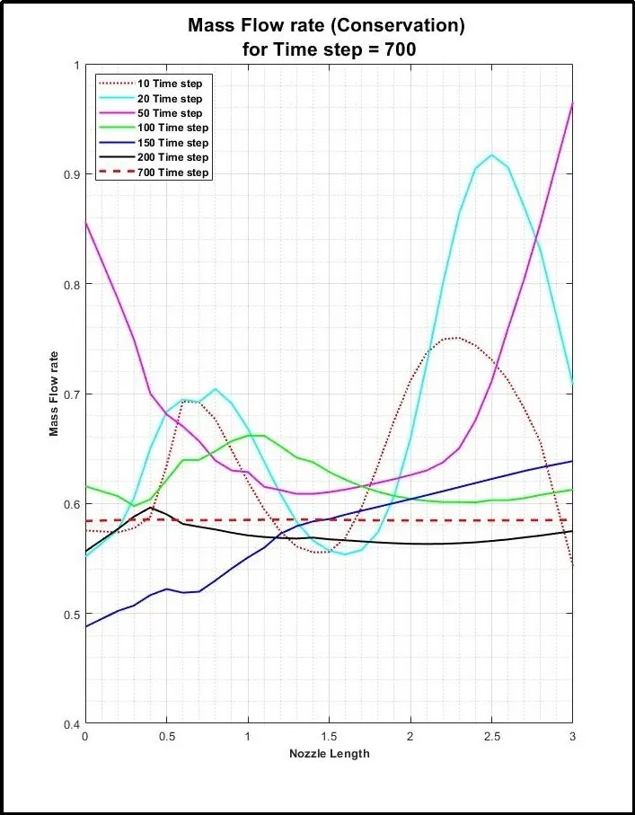
The steady-state results obtained from the time-marching solution of the governing equations in conservation form are essentially the same as those obtained using the nonconservation form.
A overview of the above graphs portray seven different curves, each for a different time during the course of the time-marching procedure. We can see at the starting at 10th time step the mass flow rate showing in red dash line, the curve almost at the initial line that we assumed at the beginning of this project. As time step increasing, the mass flow rate simply flopping around inside the nozzle due to the transient variation of the flow-field variables.
However, after 200 times steps the mass flow distribution is starting to slow down and after 700 time steps, the mass flow distribution is a straight, horizontal line across the graph. This says, the mass flow has converged to a constant, steady-state value throughout the nozzle.
We can observe above two graph of mass flow rate with conservative and non-conservative form, where we can notice the convergence of curve of results are smooth in non-conservative form.
Let us compare the steady-state variations of mass flow obtained with the nonconservation and conservation forms of the governing equations (both after 1400 time steps) this comparison we can seen in our next plot which is normalized mass flow rate distribution of both forms.
Comparison of Normalized mass flow rate distribution of both forms
We will use following codes to plot above-mentioned graph.
%==============================================================================================================%
%% Plot[5] - Comparison of Normalized mass flow rate distributions
%==============================================================================================================%

figure(5)
set(gcf, 'Position',  [10, 40, 700, 900])
plot(x,mfr_c,'color','b','linewidth',1.5)
hold on
plot(x,mfr_nc,'color','g','linewidth',1.5)
plot(x,mfr_an_x,'--','color','r','linewidth',1.5)
xlabel('Nozzle Length','fontweight','bold','fontsize',14)
ylabel('Mass Flow rate','fontweight','bold','fontsize',14)
legend({'Conservation form','Non-Conservation form','Exact '},'Location','northwest','fontweight','bold','fontsize',11)
title('Comparison of Normalized mass flow rate','fontsize',18);
grid on
grid minor
Output for above codes
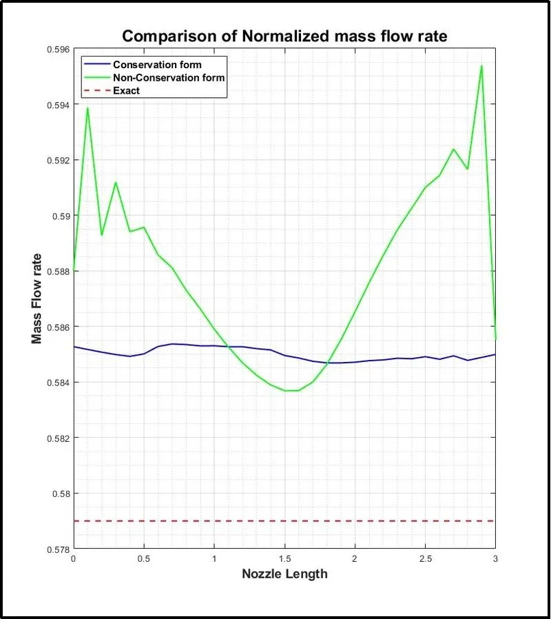
The comparison depicted in above chart, the scale of the ordinate for mass flow is greatly magnified. Here we see that the steady- state mass flow distribution predicted by the conservation form of the equations is much more satisfactory that that obtained from the nonconservation form, on two accounts:
- The conservation from gives a distribution that is much closer to being a constant. In contrast, the nonconservation results have (on the magnified scale) a sizable variation, with some spurious oscillations at both the inflow and outflow boundary. By the way, when we plot is on the normal scale these variations are not apparent, and mass flow essentially appears to be constant.
- The steady-state mass flow results obtained with the conservation form are on the whole,much closer to the exact analytical solution of rho’ A’ v’ = 0.579, shown in above graph by the dashed line
Grid independence test on the solution
Grid independence
The solution is said to be grid independent if the solution has no effect even if the number of grid points are increased once a stable solution is obtained.
To test it, let us double, triple or quadruple the no of grid points, accordingly, dt should be changed. Which will change our number of grids in between nozzle length. By doing this we will check the changes in output results.
Large variation in results means our solution is not yet grid independent and we require more number of mesh grid. On the contrary, very minimum variation is output results means we can prefer current number of mesh grid points.
To check if there any variation in our results, we first evaluate our results for following number of mesh grid points :- 31,61,91,121,151…
We are going to use following codes to print the answer in command window.
%==============================================================================================================%
%%grid independence test on the solution
%==============================================================================================================%

fprintf('For number of grid points:- %.f\n',n)
% Method 1: Define each column
T = table([0.634;rho_c(t_n);rho_nc(t_n)],[0.833;t_c(t_n);t_nc(t_n)],[0.528;p_c(t_n);p_nc(t_n)],[0.91325;v_c(t_n);v_nc(t_n)],[1;M_c(t_n);M_nc(t_n)],'VariableNames',{'rho_rho0','T_T0','p_p0','v_a0','M'},'RowName',{'[1] Exact','[2] Conservative_form','[3] Non-Conservative_form'});

% Display table
disp(T)
Output Results
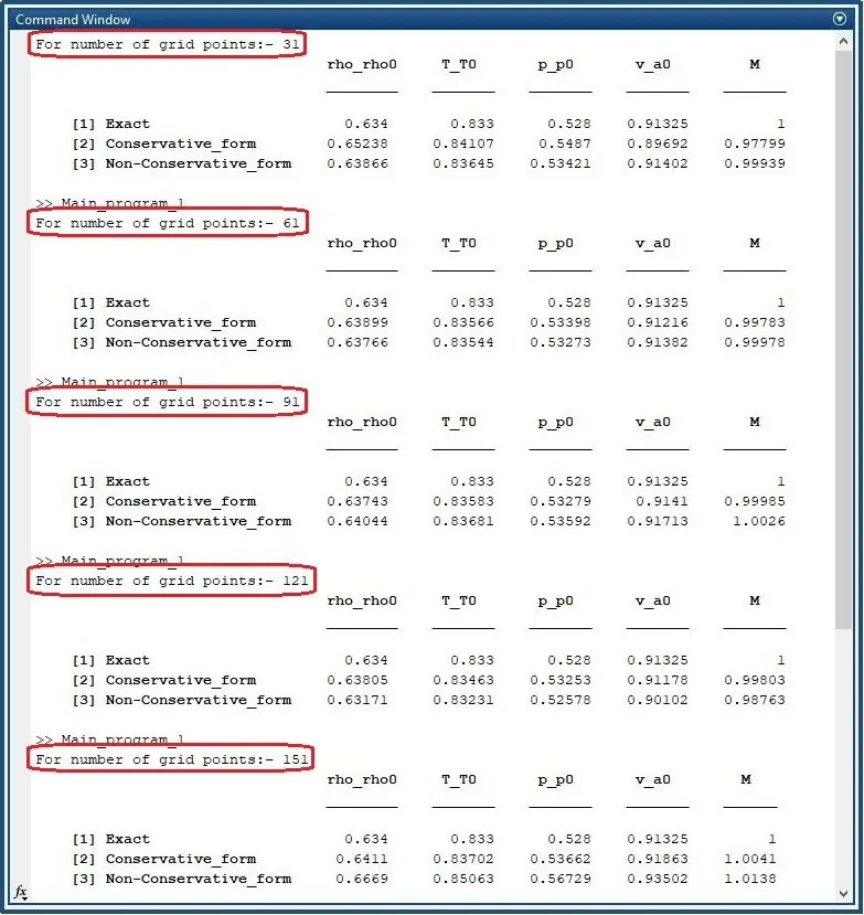
As we can see above data, there is no significant changes in the values are obtained even after making the mesh fine by multiplying the number of grid points for several number of times. Hence, we can get our reliable result with 31 grid points.
Conclusion:-
The results obtained after 1400 time steps, after a quick comparison of the numbers in final result for conservation form and nonconservation form, we conclude that , for all practical purpose, both forms of the governing equations give the same results. This is as it should be; the flow problem studied in both is the isentropic, subsonic-supersonic flow through a nozzle, and for such a flow the choice of the form of equations is not important.
However, after reading the Jhon D Anderson text book, we came to know, an important numerical distinction between the nonconservation and conservation forms of the equation is related to problems dealing with shock capturing, although we did not capture any shocks in this project.
Overall, the all results are almost same, except that the conservation from yielded a slightly better mass flow distribution.
Reference:-
Book - Computational Fluid Dynamics The Basics with Applications - Jhon D Anderson jr.
Complete Nonconservative function program
function [rho_nc v_nc t_nc p_nc mfr_nc M_nc drhodt dvdt dtdt] = non_conservation(n,x,t_n,dx,gamma,dt_nc,rho_nc,t_nc,v_nc,a)

rho_old = rho_nc;
v_old = v_nc;
t_old = t_nc;

%% Predictor method

for j = 2:n-1

    dvdx = (v_nc(j+1)-v_nc(j))/dx;
    drhodx = (rho_nc(j+1)-rho_nc(j))/dx;
    dtdx = (t_nc(j+1)-t_nc(j))/dx;
    dlogadx = (log(a(j+1))-log(a(j)))/dx;


    % Continuty Equation
    drhodt_p(j) = -rho_nc(j)*dvdx-rho_nc(j)*v_nc(j)*dlogadx - v_nc(j)*drhodx;


    % Momentum Equation
    dvdt_p(j) = -v_nc(j)*dvdx-(1/gamma)*(dtdx + (t_nc(j)/rho_nc(j))*drhodx);


    % Energy Equation
    dtdt_p(j) = -v_nc(j)*dtdx - ((gamma-1)*t_nc(j))*(dvdx + v_nc(j)*dlogadx);


    %% solution update
    rho_nc(j) = rho_nc(j) + drhodt_p(j)*dt_nc;
    v_nc(j) = v_nc(j) + dvdt_p(j)*dt_nc;
    t_nc(j) = t_nc(j) + dtdt_p(j)*dt_nc;

end


%% Corrector method
for j = 2:n-1
    dvdx = (v_nc(j)-v_nc(j-1))/dx;
    drhodx = (rho_nc(j)-rho_nc(j-1))/dx;
    dtdx = (t_nc(j)-t_nc(j-1))/dx;
    dlogadx = (log(a(j))-log(a(j-1)))/dx;


    % Continuty equation
    drhodt_c(j) = -rho_nc(j)*dvdx -rho_nc(j)*v_nc(j)*dlogadx - v_nc(j)*drhodx;

    % Momentum equation
    dvdt_c(j) = -v_nc(j)*dvdx -(1/gamma)*(dtdx + (t_nc(j)/rho_nc(j))*drhodx);

    % Energy Equation
    dtdt_c(j) = -v_nc(j)*dtdx -(gamma-1)*t_nc(j)*(dvdx + v_nc(j)*dlogadx);

end


% Compute the average time derivative
drhodt = 0.5*(drhodt_p + drhodt_c);
dvdt = 0.5*(dvdt_p + dvdt_c);
dtdt = 0.5*(dtdt_p + dtdt_c);


%% final solution Update
for i = 2:n-1
    rho_nc(i) = rho_old(i) + drhodt(i)*dt_nc;
    v_nc(i) = v_old(i) + dvdt(i)*dt_nc;
    t_nc(i) = t_old(i) + dtdt(i)*dt_nc;
end


%% Apply the boundary conditions
% Inlet
v_nc(1) = 2*v_nc(2) - v_nc(3);

% Outlet
v_nc(n) = 2*v_nc(n-1) - v_nc(n-2);
rho_nc(n) = 2*rho_nc(n-1) - rho_nc(n-2);
t_nc(n) = 2*t_nc(n-1) - t_nc(n-2);

% Pressure
p_nc = rho_nc.*t_nc;

% Mass Flow rate
mfr_nc = rho_nc.*a.*v_nc;

% Mach Number
M_nc = v_nc./(t_nc.^0.5);


end
Complete conservative function program
function [rho_c v_c t_c p_c mfr_c M_c dU1dt dU2dt dU3dt] = conservation(n,x,t_n,dx,gamma,dt_c,rho_c,t_c,v_c,a)

% solution terms
U1 = rho_c.*a;
U2 = rho_c.*a.*v_c;
U3 = U1.*((t_c/(gamma-1))+(gamma/2).*(v_c.^2));

U1_old = U1;
U2_old = U2;
U3_old = U3;


%% Predictor method
for j = 2:n-1

    F1 = U2;
    F2 = ((U2.^2)./U1)+(((gamma-1)/gamma)*(U3-((gamma/2)*((U2.^2)./U1))));
    F3 = ((gamma*U2.*U3)./U1)-(gamma*(gamma-1)*(U2.^3))./(2*U1.^2);


    j2(j) =  (1/gamma)*rho_c(j).*t_c(j).*((a(j+1)-a(j))/dx);

    %% Predictor
    % Continuty Equation
    dU1dt_p(j) = -((F1(j+1)-F1(j))/dx);

    % Momentum Equation
    dU2dt_p(j) = -((F2(j+1)-F2(j))/dx)+j2(j);

    % Energy Equation
    dU3dt_p(j) = -((F3(j+1)-F3(j))/dx);


    %% solution update
    U1(j) = U1(j) + dU1dt_p(j)*dt_c;
    U2(j) = U2(j) + dU2dt_p(j)*dt_c;
    U3(j) = U3(j) + dU3dt_p(j)*dt_c;

end

rho_c = U1./a;
v_c = U2./U1;
t_c = (gamma -1)*((U3./U1)-((gamma*v_c.^2)/2));


%% Corrector method
for j = 2:n-1

    F1 = U2;
    F2 = ((U2.^2)./U1)+(((gamma-1)/gamma)*(U3-(gamma*U2.^2)./(2*U1)));
    F3 = ((gamma*U2.*U3)./U1)-((gamma*(gamma-1)/2)*((U2.^3)./(U1.^2)));

    j2(j) =  (1/gamma)*rho_c(j).*t_c(j).*((a(j)-a(j-1))/dx);


    %% Corrector method
    % Continuty Equation
    dU1dt_c(j) = -((F1(j)-F1(j-1))/dx);

    % Momentum Equation
    dU2dt_c(j) = -((F2(j)-F2(j-1))/dx)+j2(j);

    % Energy Equation
    dU3dt_c(j) = -((F3(j)-F3(j-1))/dx);

end

% Compute the average time derivative
dU1dt = 0.5*(dU1dt_p + dU1dt_c);
dU2dt = 0.5*(dU2dt_p + dU2dt_c);
dU3dt = 0.5*(dU3dt_p + dU3dt_c);


%% final solution Update
for i = 2:n-1
    U1(i) = U1_old(i) + dU1dt(i)*dt_c;
    U2(i) = U2_old(i) + dU2dt(i)*dt_c;
    U3(i) = U3_old(i) + dU3dt(i)*dt_c;
end


%% Apply the boundary conditions
% Inlet
U1(1) = rho_c(1)*a(1);
U2(1) = 2*U2(2) - U2(3);
U3(1) = U1(1)*((t_c(1)./(gamma-1))+((gamma/2)*v_c(1).^2));

% Outlet
U1(n) = 2*U1(n-1) - U1(n-2);
U2(n) = 2*U2(n-1) - U2(n-2);
U3(n) = 2*U3(n-1) - U3(n-2);

% Corrected values
rho_c = U1./a;
v_c = U2./U1;
t_c = (gamma -1)*((U3)./(U1)-(gamma/2)*(v_c.^2));

% Pressure
p_c = rho_c.*t_c;

% Mass Flow rate
mfr_c = rho_c.*a.*v_c;

% Mach Number
M_c = v_c./((t_c).^0.5);


end
Complete Main Program
clear all       % Clear all Variables from memory
close all       % close all charts and figures
clc             % clear command window


%% Inputs
n = 31;
x = linspace(0,3,n);
dx = x(2)-x(1);
gamma = 1.4;

% Area
a = 1+2.2*(x-1.5).^2;
t_n = find(a==1);


%% Calculate initial profile Conservative form
for i = 1:length(x)
    if x(i)<=0.5
        rho_c(i)=1;
        t_c(i)=1;
    elseif x(i)>=0.5 && x(i)<=1.5
        rho_c(i) = 1-0.366*(x(i)-0.5);
        t_c(i) = 1-0.167*(x(i)-0.5);
    elseif x(i)>=1.5 && x(i)<=3
        rho_c(i) = 0.634-0.3879*(x(i)-1.5);
        t_c(i) = 0.833-0.3507*(x(i)-1.5);
    end
end
v_c = 0.59./(rho_c.*a);


%% Initial profile for Non-Conservative form
rho_nc = 1-0.3146*x;
t_nc = 1-0.2314*x;
v_nc = (0.1+1.09*x).*t_nc.^0.5;


%% No of Time step
nt = 1400;
time_range=linspace(1,nt,nt);

% Time Step
CFL=0.5;
dt_c = min(CFL.*(dx./(t_c.^0.5+v_c)));
dt_nc = min(CFL.*(dx./(t_nc.^0.5+v_nc)));


%% analytical calculations
a_an = a(t_n).*ones(1,nt);
rho_an = 0.634*ones(1,nt);
v_an = 0.579./(rho_an.*a_an);
t_an = 0.833*ones(1,nt);
p_an = 0.528*ones(1,nt);
% Mass flow rate for length of nt
mfr_an = 0.579*ones(1,nt);
% Mass Flow rate for length of x
mfr_an_x = 0.579*ones(1,length(x));
% Mach Number
M_an = v_an./(t_an.^0.5);


%% Plotting(Non-Conservative form)
tic
for k = 1:nt

    [rho_nc v_nc t_nc p_nc mfr_nc M_nc drhodt dvdt dtdt] = non_conservation(n,x,t_n,dx,gamma,dt_nc,rho_nc,t_nc,v_nc,a);


    %==============================================================================================================%
    %% Plot[1] - Plotting Steady-State Distribution of Primitive Variables for Non- Conservation form
    %           for Non- Conservation form
    %==============================================================================================================%

    figure(1);
    set(gcf, 'Position',  [10, 40, 1400, 1000])

    subplot(3,2,1)
    plot(x,rho_nc,'color','g','linewidth',1.5)
    axis([0 3 0 1.4])
    xlabel('Nozzle Length','fontweight','bold','fontsize',9)
    ylabel('Density','fontweight','bold','fontsize',9)
    heading = sprintf('Steady State Distribution of Density \nInside The Nozzle \nfor Time step = %d',k);
    title(heading,'fontsize',10);
    grid on
    grid minor

    subplot(3,2,2)
    plot(x,v_nc,'color','b','linewidth',1.5)
    axis([0 3 0 2.2])
    xlabel('Nozzle Length','fontweight','bold','fontsize',9)
    ylabel('Velocity','fontweight','bold','fontsize',9)
    heading = sprintf('Steady State Distribution of Velocity \nInside The Nozzle \nfor Time step = %d',k);
    title(heading,'fontsize',10);
    grid on
    grid minor

    subplot(3,2,3)
    plot(x,t_nc,'color','k','linewidth',1.5)
    axis([0 3 0 1.2])
    xlabel('Nozzle Length','fontweight','bold','fontsize',9)
    ylabel('Temperature','fontweight','bold','fontsize',9)
    heading = sprintf('Steady State Distribution of Temperature \nInside The Nozzle \nfor Time step = %d',k);
    title(heading,'fontsize',10);
    grid on
    grid minor

    subplot(3,2,4)
    plot(x,p_nc,'color','m','linewidth',1.5)
    axis([0 3 -0.1 1.5])
    xlabel('Nozzle Length','fontweight','bold','fontsize',9)
    ylabel('Pressure','fontweight','bold','fontsize',9)
    heading = sprintf('Steady State Distribution of Pressure \nInside The Nozzle \nfor Time step = %d',k);
    title(heading,'fontsize',10);
    grid on
    grid minor

    subplot(3,2,5)
    plot(x,mfr_nc,'color','r','linewidth',1.5)
    axis([0 3 -0.1 2.5])
    xlabel('Nozzle Length','fontweight','bold','fontsize',9)
    ylabel('Mass Flow rate','fontweight','bold','fontsize',9)
    heading = sprintf('Steady State Distribution of Mass Flow rate \nInside The Nozzle \nfor Time step = %d',k);
    title(heading,'fontsize',10);
    grid on
    grid minor

    subplot(3,2,6)
    plot(x,M_nc,'color','c','linewidth',1.5)
    axis([0 3 -0.1 4])
    xlabel('Nozzle Length','fontweight','bold','fontsize',9)
    ylabel('Mach Number','fontweight','bold','fontsize',9)
    heading = sprintf('Steady State Distribution of Mach Number \nInside The Nozzle \nfor Time step = %d',k);
    title(heading,'fontsize',10);
    grid on
    grid minor


    %==============================================================================================================%
    %% Plot[3] - Variation of Mass flow rate distribution inside the nozzle at different time steps
    %           for Non-conservation form
    %==============================================================================================================%

    figure(3)
    set(gcf, 'Position',  [10, 40, 700, 900])
    if k == 1
        plot(x,mfr_nc,':','color','r','linewidth',1.5)
        hold on
    elseif k == 20
        plot(x,mfr_nc,'color','c','linewidth',1.5)
    elseif k == 50
        plot(x,mfr_nc,'color','m','linewidth',1.5)
    elseif k == 100
        plot(x,mfr_nc,'color','g','linewidth',1.5)
    elseif k == 150
        plot(x,mfr_nc,'color','b','linewidth',1.5)
    elseif k == 200
        plot(x,mfr_nc,'color','k','linewidth',1.5)
    elseif k == 700
        plot(x,mfr_nc,'--','color','r','linewidth',2)
        legend({'10 Time step','20 Time step','50 Time step','100 Time step','150 Time step','200 Time step','700 Time step'},'fontweight','bold','fontsize',9)
        xlabel('Nozzle Length','fontweight','bold','fontsize',10)
        ylabel('Mass Flow rate','fontweight','bold','fontsize',10)
        heading = sprintf('Mass Flow rate (non-conservation) \nfor Time step = %d',k);
        title(heading,'fontsize',16);
        grid on
        grid minor
        hold off
    end


    %% Residuals
    residuals_1_nc(k) = max(abs(drhodt));
    residuals_2_nc(k) = max(abs(dvdt));
    residuals_3_nc(k) = max(abs(dtdt));


    %% Throat Values
    rho_nc_throat(k) = rho_nc(t_n);
    v_nc_throat(k) = v_nc(t_n);
    t_nc_throat(k) = t_nc(t_n);
    p_nc_throat(k) = p_nc(t_n);
    mfr_nc_throat(k) = mfr_nc(t_n);
    M_nc_throat(k) = M_nc(t_n);
end
Time_nc = toc


%% Plotting(Conservative form)
tic
for k = 1:nt

    [rho_c v_c t_c p_c mfr_c M_c dU1dt dU2dt dU3dt] = conservation(n,x,t_n,dx,gamma,dt_c,rho_c,t_c,v_c,a);


    %==============================================================================================================%
    %% Plot[2] - Plotting Steady-State Distribution of Primitive Variables for Conservation form
    %           for Conservation form
    %==============================================================================================================%

    figure(2);
    set(gcf, 'Position',  [10, 40, 1400, 1000])

    subplot(3,2,1)
    plot(x,rho_c,'color','g','linewidth',1.5)
    axis([0 3 0 1.4])
    xlabel('Nozzle Length','fontweight','bold','fontsize',9)
    ylabel('Density','fontweight','bold','fontsize',9)
    heading = sprintf('Steady State Distribution of Density \nInside The Nozzle \nfor Time step = %d',k);
    title(heading,'fontsize',10);
    grid on
    grid minor

    subplot(3,2,2)
    plot(x,v_c,'color','b','linewidth',1.5)
    axis([0 3 0 2.2])
    xlabel('Nozzle Length','fontweight','bold','fontsize',9)
    ylabel('Velocity','fontweight','bold','fontsize',9)
    heading = sprintf('Steady State Distribution of Velocity \nInside The Nozzle \nfor Time step = %d',k);
    title(heading,'fontsize',10);
    grid on
    grid minor

    subplot(3,2,3)
    plot(x,t_c,'color','k','linewidth',1.5)
    axis([0 3 0 1.2])
    xlabel('Nozzle Length','fontweight','bold','fontsize',9)
    ylabel('Temperature','fontweight','bold','fontsize',9)
    heading = sprintf('Steady State Distribution of Temperature \nInside The Nozzle \nfor Time step = %d',k);
    title(heading,'fontsize',10);
    grid on
    grid minor

    subplot(3,2,4)
    plot(x,p_c,'color','m','linewidth',1.5)
    axis([0 3 -0.1 1.5])
    xlabel('Nozzle Length','fontweight','bold','fontsize',9)
    ylabel('Pressure','fontweight','bold','fontsize',9)
    heading = sprintf('Steady State Distribution of Pressure \nInside The Nozzle \nfor Time step = %d',k);
    title(heading,'fontsize',10);
    grid on
    grid minor

    subplot(3,2,5)
    plot(x,mfr_c,'color','r','linewidth',1.5)
    axis([0 3 -0.1 2.5])
    xlabel('Nozzle Length','fontweight','bold','fontsize',9)
    ylabel('Mass Flow rate','fontweight','bold','fontsize',9)
    heading = sprintf('Steady State Distribution of Mass Flow rate \nInside The Nozzle \nfor Time step = %d',k);
    title(heading,'fontsize',10);
    grid on
    grid minor

    subplot(3,2,6)
    plot(x,M_c,'color','c','linewidth',1.5)
    axis([0 3 -0.1 4])
    xlabel('Nozzle Length','fontweight','bold','fontsize',9)
    ylabel('Mach Number','fontweight','bold','fontsize',9)
    heading = sprintf('Steady State Distribution of Mach Number \nInside The Nozzle \nfor Time step = %d',k);
    title(heading,'fontsize',10);
    grid on
    grid minor


    %==============================================================================================================%
    %% Plot[4] - Variation of Mass flow rate distribution inside the nozzle at different time steps
    %           for Conservation form
    %==============================================================================================================%

    figure(4)
    set(gcf, 'Position',  [10, 40, 700, 900])
    if k == 10
        plot(x,mfr_c,':','color','r','linewidth',1.5)
        hold on
    elseif k == 20
        plot(x,mfr_c,'color','c','linewidth',1.5)
    elseif k == 50
        plot(x,mfr_c,'color','m','linewidth',1.5)
    elseif k == 100
        plot(x,mfr_c,'color','g','linewidth',1.5)
    elseif k == 150
        plot(x,mfr_c,'color','b','linewidth',1.5)
    elseif k == 200
        plot(x,mfr_c,'color','k','linewidth',1.5)
    elseif k == 700
        plot(x,mfr_c,'--','color','r','linewidth',2)
        legend({'10 Time step','20 Time step','50 Time step','100 Time step','150 Time step','200 Time step','700 Time step'},'Location','northwest','fontweight','bold','fontsize',9)
        xlabel('Nozzle Length','fontweight','bold','fontsize',10)
        ylabel('Mass Flow rate','fontweight','bold','fontsize',10)
        heading = sprintf('Mass Flow rate (Conservation) \nfor Time step = %d',k);
        title(heading,'fontsize',16);
        grid on
        grid minor
        hold off
    end


    %% Residuals
    residuals_1_c(k) = max(abs(dU1dt));
    residuals_2_c(k) = max(abs(dU2dt));
    residuals_3_c(k) = max(abs(dU3dt));


    %% Throat Values
    rho_c_throat(k) = rho_c(t_n);
    v_c_throat(k) = v_c(t_n);
    t_c_throat(k) = t_c(t_n);
    p_c_throat(k) = p_c(t_n);
    mfr_c_throat(k) = mfr_c(t_n);
    M_c_throat(k) = M_c(t_n);
end
Time_c = toc


%==============================================================================================================%
%% Plot[5] - Comparison of Normalized mass flow rate distributions
%==============================================================================================================%

figure(5)
set(gcf, 'Position',  [10, 40, 700, 900])
plot(x,mfr_c,'color','b','linewidth',1.5)
hold on
plot(x,mfr_nc,'color','g','linewidth',1.5)
plot(x,mfr_an_x,'--','color','r','linewidth',1.5)
xlabel('Nozzle Length','fontweight','bold','fontsize',14)
ylabel('Mass Flow rate','fontweight','bold','fontsize',14)
legend({'Conservation form','Non-Conservation form','Exact '},'Location','northwest','fontweight','bold','fontsize',11)
title('Comparison of Normalized mass flow rate','fontsize',18);
grid on
grid minor


%==============================================================================================================%
%% Plot[6] - Timewise variations of the density, temperature, pressure, and Mach number at the nozzle throat
%==============================================================================================================%

figure(6);
set(gcf, 'Position',  [10, 40, 1400, 1000])

subplot(3,2,1)
plot(time_range,rho_c_throat,'color','b','linewidth',1.5)
hold on
plot(time_range,rho_nc_throat,'color','g','linewidth',1.5)
plot(time_range,rho_an,'color','k','linewidth',1.5)
legend({'Conservation form','Non-Conservation form','Exact '},'fontweight','bold','fontsize',8)
xlabel('Number of time steps','fontweight','bold','fontsize',9)
ylabel('Density','fontweight','bold','fontsize',9)
heading = sprintf('Timewise variations of the Density \nat the nozzle throat');
title(heading,'fontsize',10);
grid on
grid minor

subplot(3,2,2)
plot(time_range,v_c_throat,'color','b','linewidth',1.5)
hold on
plot(time_range,v_nc_throat,'color','g','linewidth',1.5)
plot(time_range,v_an,'color','k','linewidth',1.5)
legend({'Conservation form','Non-Conservation form','Exact '},'fontweight','bold','fontsize',8)
xlabel('Number of time steps','fontweight','bold','fontsize',9)
ylabel('Velocity','fontweight','bold','fontsize',9)
heading = sprintf('Timewise variations of the Velocity \nat the nozzle throat');
title(heading,'fontsize',10);
grid on
grid minor

subplot(3,2,3)
plot(time_range,t_c_throat,'color','b','linewidth',1.5)
hold on
plot(time_range,t_nc_throat,'color','g','linewidth',1.5)
plot(time_range,t_an,'color','k','linewidth',1.5)
legend({'Conservation form','Non-Conservation form','Exact '},'fontweight','bold','fontsize',8)
xlabel('Number of time steps','fontweight','bold','fontsize',9)
ylabel('Temperature','fontweight','bold','fontsize',9)
heading = sprintf('Timewise variations of the Temperature \nat the nozzle throat');
title(heading,'fontsize',10);
grid on
grid minor

subplot(3,2,4)
plot(time_range,p_c_throat,'color','b','linewidth',1.5)
hold on
plot(time_range,p_nc_throat,'color','g','linewidth',1.5)
plot(time_range,p_an,'color','k','linewidth',1.5)
legend({'Conservation form','Non-Conservation form','Exact '},'fontweight','bold','fontsize',8)
xlabel('Number of time steps','fontweight','bold','fontsize',9)
ylabel('Pressure','fontweight','bold','fontsize',9)
heading = sprintf('Timewise variations of the Pressure \nat the nozzle throat');
title(heading,'fontsize',10);
grid on
grid minor

subplot(3,2,5)
plot(time_range,mfr_c_throat,'color','b','linewidth',1.5)
hold on
plot(time_range,mfr_nc_throat,'color','g','linewidth',1.5)
plot(time_range,mfr_an,'color','k','linewidth',1.5)
legend({'Conservation form','Non-Conservation form','Exact '},'fontweight','bold','fontsize',8)
xlabel('Number of time steps','fontweight','bold','fontsize',9)
ylabel('Mass Flow rate','fontweight','bold','fontsize',9)
heading = sprintf('Timewise variations of the Mass Flow rate \nat the nozzle throat');
title(heading,'fontsize',10);
grid on
grid minor

subplot(3,2,6)
plot(time_range,M_c_throat,'color','b','linewidth',1.5)
hold on
plot(time_range,M_nc_throat,'color','g','linewidth',1.5)
plot(time_range,M_an,'color','k','linewidth',1.5)
legend({'Conservation form','Non-Conservation form','Exact '},'fontweight','bold','fontsize',8)
xlabel('Number of time steps','fontweight','bold','fontsize',9)
ylabel('Mach Number','fontweight','bold','fontsize',9)
heading = sprintf('Timewise variations of the Mach Number \nat the nozzle throat');
title(heading,'fontsize',10);
grid on
grid minor


%==============================================================================================================%
%% Plot[7] - Timewise variations in residual
%==============================================================================================================%

figure(7)
subplot(1,2,1)
set(gcf, 'Position',  [10, 40, 1400, 900])
plot(time_range,residuals_1_c,'color','r','linewidth',1.5)
hold on
plot(time_range,residuals_2_c,'color','b','linewidth',1.5)
plot(time_range,residuals_3_c,'color','g','linewidth',1.5)
xlabel('Number of time steps','fontweight','bold','fontsize',12)
ylabel('Residual','fontweight','bold','fontsize',12)
legend({'residual for dU_1/dt','residual for dU_2/dt','residual for dU_3/dt'},'fontweight','bold','fontsize',11)
title('Timewise variations in residual (Conservation form)','fontsize',16);
grid on
grid minor

subplot(1,2,2)
plot(time_range,residuals_1_nc,'color','r','linewidth',1.5)
hold on
plot(time_range,residuals_2_nc,'color','b','linewidth',1.5)
plot(time_range,residuals_3_nc,'color','g','linewidth',1.5)
xlabel('Number of time steps','fontweight','bold','fontsize',12)
ylabel('Residual','fontweight','bold','fontsize',12)
legend({'residual for drho/dt','residual for dv/dt','residual for dT/dt'},'fontweight','bold','fontsize',11)
title('Timewise variations in residual (Non-conservation form)','fontsize',16);
grid on
grid minor


%==============================================================================================================%
%%grid independence test on the solution
%==============================================================================================================%

fprintf('For number of grid points:- %.f\n',n)
% Method 1: Define each column
T = table([0.634;rho_c(t_n);rho_nc(t_n)],[0.833;t_c(t_n);t_nc(t_n)],[0.528;p_c(t_n);p_nc(t_n)],[0.91325;v_c(t_n);v_nc(t_n)],[1;M_c(t_n);M_nc(t_n)],'VariableNames',{'rho_rho0','T_T0','p_p0','v_a0','M'},'RowName',{'[1] Exact','[2] Conservative_form','[3] Non-Conservative_form'});

% Display table
disp(T)