Week 7 - Simulation of a 1D Super-sonic nozzle flow simulation using Macormack Method
SIMULATION OF QUASI ONE DIMENSIONAL SUPERSONIC NOZZLE FLOW USING MACCORMACK METHOD:
Problem specification:
In this challenge you are going to simulate the isentropic flow through a quasi 1D subsonic-supersonic nozzle. You will derive both the conservation and non-conservation forms of the governing equations and sovle them using the MacCormack's technique. You need to determine the steady-state temperature distribution for the flow-field variables and investigate the difference between the two forms of governing equations by comparing their solutions.
Need to show the following plots inside the report
1. Steady-state distribution of primitive variables inside the nozzle
2. Time-wise variation of the primitive variables
3. Variation of Mass flow rate distribution inside the nozzle at different time steps during the time-marching process
4. Comparison of Normalized mass flow rate distributions of both forms
Expected Results:
- Perform a grid independence test on the solution and expain all your findings.
- The code must be modular. You need to write separate functions to solve both forms.
- Discuss all the plots you are providing with observed inferences.
THEORY:
MacCormack technique:
It is an explicit finite difference technique which is second order accurate in both space and time.
Lets consider an unsteady,2-d inviscid flow
Eulers equations in non-conservative form:
Continuity: `(deltarho)/(deltat)=-(rho(deltau)/(deltax)+u(deltarho)/(deltax)+rho(deltav)/(deltay)+v(deltap)/(deltay))`------1
x-momentum:`(deltau)/(deltat)=-(u(deltau)/(deltax)+v(deltau)/(deltay)+1/rho(deltarho)/(deltax))`----------2
y-momentum:`(deltav)/(deltat)=-(u(deltav)/(deltax)+v(deltav)/(deltay)+1/rho(deltarho)/(deltay))`------------3
Energy:`(deltae)/(deltat)=-(u(deltae)/(deltax)+v(deltae)/(deltay)+P/rho(deltau)/(deltax)+P/rho(deltau)/(deltay))`--------4
In the above equation we assumed no body forces and no volumetric heat addition i.e f=0 and q=0 the above equation are hyperbolic w.r.t time we assume that flow field at the time (t) is known and we will identify at (t+Deltat).
Here we are choosing density rho as our dependent flow variable for which we are going to derive the maccormack method,
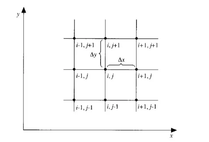
Let `(rho^(t))_(i,j)` denote the density at grid points (i,j) at the time(t) density at the same grid point at the time (t+Deltat) is given by,
`(rho^(t+Deltat))_(i,j)=(rho^(t))_(i,j)+((deltarho)/(deltat))_(av) Deltat`-------5`
Where `((deltarho)/(deltat))_(av` denotes the mean value of `(deltarho)/(deltat)` between the times(t) and (t+Deltat)
values of `((deltarho)/(deltat))_(av` is calculated to preserve second order accuracy wihtout the need to calculate values of the second order time derivative which is the term inolves a lot of algebra.
Similar relations are written for the other flow fiel variables.
`(u^(t+Deltat))_(i,j)=(u^(t))_(i,j)+((deltau)/(deltat))_(av) Deltat`-------6
`(v^(t+Deltat))_(i,j)=(v^(t))_(i,j)+((deltav)/(deltat))_(av) Deltat-------`7
`(e^(t+Deltat))_(i,j)=(e^(t))_(i,j)+((deltae)/(deltat))_(av) Deltat-------``8
From equation (5);
Average time derivative `(deltarho)/(deltat)_(av)` is obtained from a predictor and corrector method.
Predictor step:
In the continuity equation (1) discretize the spatial derivatives on the right hand side using forward difference scheme.
Predicted value of density (rho)t+DEltat from the first two terns of taylor series as follows,
`(rho^(t+Deltat))_(i,j)=(rho^(t))_(i,j)+((deltarho)/(deltat))_(i,j) Deltat`-----10
similarly:
`(u^(t+Deltat))_(i,j)=(u^(t))_(i,j)+((deltau)/(deltat))_(i,j) Deltat`----------11
`(v^(t+Deltat))_(i,j)=(v^(t))_(i,j)+((deltav)/(deltat))_(i,j) Deltat`-----------12
`(e^(t+Deltat))_(i,j)=(e^(t))_(i,j)+((deltae)/(deltat))_(i,j) Deltat------------13
In the above equations 10 to 13 numbers for the time derivative on the right hand side are obtained from the equation.
Corrector step:
In the corrector step,we use the calculated predicted value of the time derivative at the time `(t+Deltat).((deltarho)/(deltat))^(t-Deltat)_(i,j)` by substituting the values of rho,u,v into the rhs of the conitinuty equation(1) discretizing spatial derivatives by using backward difference scheme.
`(deltarho)/(deltat)=-(rho^-t+Deltat)_(i,j)((u^-t+Deltat)_(i,j)-(u^-t+Deltat)_(i-1,j))/(Deltax)+(u^-t+Deltat)_(i,j)((rho^-t+Deltat)_(i,j)-(rho^-t-Deltat)_(i-1,j))/(Deltax)+(rho^t+Deltat)_(i,j)((v^t+Deltat)_(i,j)-(v^t+Deltat)_(i-1,j))/(Deltay)+(v^t+Deltat)_(i,j)((rho^t+Deltat)_(i,j)-(rho^t+Deltat)_(i-1,j))/(Deltay)`-------14
The average value of the time derivative of density in equation (5) is obtianed from the arithmetic mean of `((deltarho)/(deltat))^t)_(i,j)` obtained in equation (9) and (deltarho)/(deltat)t+Deltat at (i,j) obtained from equation 14
this allows us to obtain the final corrected valued of density at the time (t+deltat) from equation 5
`(rho^(t+Deltat))_(i,j)=(rho^(t))_(i,j)+((deltarho)/(deltat))_(av) Deltat`
A similar procedure can be applied to calculate momentum and energy.
Let `(rho^(t))_(i,j)` denote the density at grid points (i,j) at the time(t) density at the same grid point at the time (t+Deltat) is given by,
`(rho^(t+Deltat))_(i,j)=(rho^(t))_(i,j)+((deltarho)/(deltat))_(av) Deltat`-------`
Where `((deltarho)/(deltat))_(av` denotes the mean value of `(deltarho)/(deltat)` between the times(t) and (t+Deltat)
values of `((deltarho)/(deltat))_(av` is calculated to preserve second order accuracy wihtout the need to calculate values of the second order time derivative which is the term inolves a lot of algebra.
Similar relations are written for the other flow fiel variables.
`(u^(t+Deltat))_(i,j)=(u^(t))_(i,j)+((deltau)/(deltat))_(av) Deltat`-------6
`(v^(t+Deltat))_(i,j)=(v^(t))_(i,j)+((deltav)/(deltat))_(av) Deltat-------`7
`(e^(t+Deltat))_(i,j)=(e^(t))_(i,j)+((deltae)/(deltat))_(av) Deltat-------``8
From equation (5);
Average time derivative `(deltarho)/(deltat)_(av)` is obtained from a predictor and corrector method.
Predictor step:
In the continuity equation (1) discretize the spatial derivatives on the right hand side using forward difference scheme.
Predicted value of density (rho)t+DEltat from the first two terns of taylor series as follows,
`(rho^(t+Deltat))_(i,j)=(rho^(t))_(i,j)+((deltarho)/(deltat))_(i,j) Deltat`-----10
similarly:
`(u^(t+Deltat))_(i,j)=(u^(t))_(i,j)+((deltau)/(deltat))_(i,j) Deltat`----------11
`(v^(t+Deltat))_(i,j)=(v^(t))_(i,j)+((deltav)/(deltat))_(i,j) Deltat`-----------12
`(e^(t+Deltat))_(i,j)=(e^(t))_(i,j)+((deltae)/(deltat))_(i,j) Deltat------------13
In the above equations 10 to 13 numbers for the time derivative on the right hand side are obtained from the equation.
Corrector step:
In the corrector step,we use the calculated predicted value of the time derivative at the time `(t+Deltat).((deltarho)/(deltat))^(t-Deltat)_(i,j)` by substituting the values of rho,u,v into the rhs of the conitinuty equation(1) discretizing spatial derivatives by using backward difference scheme.
`(deltarho)/(deltat)=-(rho^-t+Deltat)_(i,j)((u^-t+Deltat)_(i,j)-(u^-t+Deltat)_(i-1,j))/(Deltax)+(u^-t+Deltat)_(i,j)((rho^-t+Deltat)_(i,j)-(rho^-t-Deltat)_(i-1,j))/(Deltax)+(rho^t+Deltat)_(i,j)((v^t+Deltat)_(i,j)-(v^t+Deltat)_(i-1,j))/(Deltay)+(v^t+Deltat)_(i,j)((rho^t+Deltat)_(i,j)-(rho^t+Deltat)_(i-1,j))/(Deltay)`-------14
The average value of the time derivative of density in equation (5) is obtianed from the arithmetic mean of `((deltarho)/(deltat))^t)_(i,j)` obtained in equation (9) and (deltarho)/(deltat)t+Deltat at (i,j) obtained from equation 14
this allows us to obtain the final corrected valued of density at the time (t+deltat) from equation 5
`(rho^(t+Deltat))_(i,j)=(rho^(t))_(i,j)+((deltarho)/(deltat))_(av) Deltat`
A similar procedure can be applied to calculate momentum and energy.
Numerical solution of quasi one dimensional supersonic nozzle flow using macCormack method:
Assumptions:the flow at the inlet to the nozzle comes from a reservoir where the pressure,temperature and density are denoted by teh cross sectional area of the reservior is large (A.infinity)and hence velocity is very small (V>0).
We consider the steady, isentropic flow through a convergent-divergent nozzle as sketched in The flow at the inlet to the nozzle comes from a reservoir where the pressure and temperature are denoted by p0 , and To, respectively. Thcross-sectional area of the reservoir is large ( theoretically, A >infinity ), and hence the velocity is very small ( V> O). Thus, Po and T0 are the stagnation values,_ or total
pressure and total temperature, respectively. The flow expands 1sentrop1cally. to supersonic speeds at the nozzle exit, where the exit pressure, temperature, velocity and Mach number are denoted by Pe, Te, V.,, and Me, respectlvely. The flow IS locally subsonic in the convergent section if the nozzle, some at the throat (minimum area), and supersonic at the d1vergent section. flow
(M = 1) at the throat means that the local velocity at this location 1s equal to the local speed of sound.
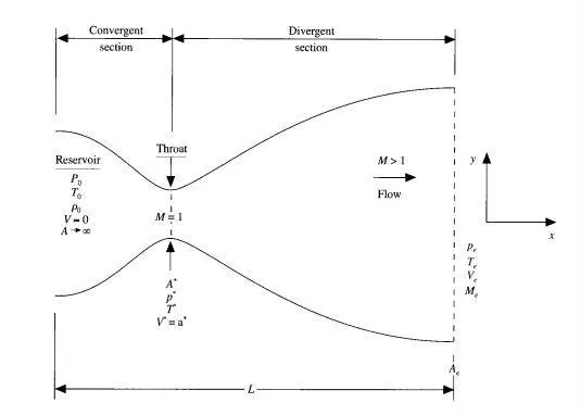
Using an asterisk to denote sonic flow values, we have at the throat V = V* = a*. Similarly, the sonic flow values of pressure and temperature are denoted by p* and T*, respectively. The area of the sonic throat is denoted by A*. We assume that at a given section, where the cross-sectional area is A, the flow properties are uniform across that section. Hence, although the area of the nozzle changes as a function of distance along the nozzle, x, and therefore in reality the flow field is two-dimensional (the flow varies in.the two-dimensional .ry space), we make the assumption that the flow properties-vary only with x; this is tantamount to assuming uniform flow properties across any given cross section. Such flow is defined as quasi-one-dimensional flow. The governing continuity, momentum, and energy equations for this quasione-dimensional, steady, isentropic flow can be expressed, respectively, as
Continuity:
Conservative form: `(delta)/(deltat)(rhoA)+(delta)/(deltax)(rhoAV)=0`------16
Non conservative form:(delta)/(deltat)(rhoA)+V(delta)/(deltax)(rhoA)=-rhoA(deltaV)/(deltax)---------17
Momentum:
Conservtaive:`(delta)/(deltat)(rhoAV)+(delta)/(deltax)(rhoAV^2)=-A(deltaP)/(deltax)`-----------18
Non conservative form:`rho(deltaV)/(deltat)+rhoV(deltaV)/(deltax)=-R[rho(deltaT)/(deltax)-T(deltarho)/(deltax)]`-------19
Energy:
conservative:`(delta)/deltat)(rhoeA)+(delta)/(deltax)(rhoeVA)=-P(delta)/(deltax)(AV)`--------20
Non conservative:`rho(deltae)/(deltat)+rhoV(deltae)/(deltax)=-P(deltaV)/(deltax)-PV(delta)/(deltax)(lnA)`---------21
The reason for obtaining the energy equation in the form of equation 21 is that for a calorifically perfect gas it leads directly to form of the energy equation in terms of temperature T.for our solution of the quasi one dimenisonal nozzle flow of a calorifically perfect gas this is a fundamental variable T and therefore it is conveniemt to deal with it as the primary dependent variable in the energy section.
For a calorically perfect gas e= CvT
hence the energy equation of conservative and non conservative form from equation 20 and 21 becomes
`conservative form:C_V(delta)/(deltat)(rhoTA)+(delta)/(deltax)(rhoTVA)=-P(delta)/(deltax)(AV)`
`Non conservative:rhoC_v(deltaT)/(deltat)+rhoV(deltaT)/(deltax)=-P(deltaV)/(deltax)-PV(delta)/(deltax)(lnA)`
Momentum:
`conservtaive:(delta)/(deltat)(rhoAV)+(delta)/(deltax)(rhoAV^2)=-A[R(rho(deltaT)/(deltax)+T(deltaP)/(deltax)-----------26`
`non conservative form:rho(deltaV)/(deltat)+rhoV(deltaV)/(deltax)=-R[rho(deltaT)/(deltax)-T(deltarho)/(deltax)]-------27`
Non-dimenisonal variables:
Dimensionless temperature T' =T/To
Dimenisonless density rho'=rho/rho0
where To and rho0 represents reservior temperature and density respectively.
dimensionless length x'=x/L
where L represents length of nozzle.
speed pf sound in the reservior ao=squareroot of gammaRTo.
dimensionless velocity V'=V/a0
dimensionaless time t'=T/L/ao.
dimensionless area A'=A/A local area /sonic throat area.
Returning to our derived conitinuity momentum adn energy equations and substituting non-dimensional variables.
Continuity:
conservative form:`(delta)/(deltat')(rho'A')+(delta)/(deltax')(rho'A'V')=0`-----30
non-conservative:`(deltarho')/(deltat')=-P'(deltaV')/(deltax')-rho'V'(delta)/(deltax')(lnA')-V'(deltarho')/(deltax')`------31
Momentum:
Conservative form:`(delta)/(deltat')(rho'A'V')+(delta)/(deltax')[rho'A'(V')^2+(1)/(gamma)rho'A']=(1)/(gamma)rho'(deltaA')/(deltax')`-----32
Non conservative form:`(deltaV')/(deltat)=-V'(deltaV')/(deltax')-(1)/(gamma)[(deltaT')/(deltax')+(T')/(rho')(deltarho')/(deltax')]`---33
Energy:
conservative:`(delta)/(deltat')[rho'((e')/(gamma-1)+(gamma)/2(V')^2)A')]+(delta)/(deltax')[rho'((e')/(gamma-1)+(gamma)/2(V')^2)V'A'+rho'AV']=0`------------34
Non conservative:`(deltaT')/(deltat')=-V'(deltaT')/(deltax')-(gamma-1)T'[(deltaV')/(deltax')+(lnA')V'(delta)/(deltax')]`-------35
Meshing:
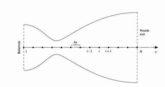
The first grid point labeled point 1 is assumed to be in the reservior points are evenly distributed along the x-axis with Deltax grid spacing point(i) is simply an arbitary grid point with points(i-1) and (i+1) as the adjacent points
For this particular problem we are taking the number of grid points to be 31 and 61(as to run the grid dependence test)
Average time derivatives:
`(rho^(t+Deltat))_(i,)=(rho^(t))_(i,)+((deltarho)/(deltat))^t_(av) Deltat`
`(V^(t+Deltat))_(i,)=(V^(t))_(i,)+((deltaV)/(deltat))^t_(av) Deltat`
`(T^(t+Deltat))_(i,)=(T^(t))_(i,)+((deltaT)/(deltat))^t_(av) Deltat`
Initial conditions(at the time =0);
Depending on the values of x-node we are setting up the values for rho,V and T.
rho=1-0.3146x.
V=1-0.2314x
T=(0.1=1.09x)T^0.5.
Nozzle shape:
For area(A),we are going to set up a profile.
A=1+2.2(x-1.5)^2 0<x<3.
Mach number:
M=V/root of T.
Calculation of time step:
For both non-conservative and conservative form of governing equation we are going to take time step.
`Deltat=c(Deltax)/(a+v)`-----40
where C=courant number
V=local flow velocity
a=locl speed of sound.
for an eplicit numerical solution to be stable C<1 ,here we are taking C=0.5.
Equation 40 is the CFL criterion for a one dimensional flow along with C<1 it simply states that delta t must be less than or at best equal to the time taken by a sound wave to move from one grid point to the next.
Deltax is the same throughout the flow,but both V' and a are variables.hence at a given grid points ata given time step.
`(Deltat^t)_(i)=C(Deltax)/((a^t)_i+(V^t)_i`
And at an adjacent grid point:
`(Deltat^t)_(i+1)=C(Deltax)/((a^t)_(i+1)+(V^t)_(i+1)`
Boundary conditions:
subsonic inflow boundary (at node1 )
We must allow one varibale to float,we choose the velocity V because on a physical basis we know that the mass flow through the nozzle must be allowed to adjust to the proper steady state and allowing V to float makes the complete sense as part of this adjustment
V1=2V2-V3
Density and temperature are fixed (independent of time)
rho1=1 and T1=1
Supersonic outflow boundary(at node N)
we must allow all flow field variables to float.
Vn=2Vn-1-Vn-2
rhon=2rhon-1-rhon-2
Tn=2Tn-1-Tn-2
Conservative form of governing equations:
Governing equations for quasi-one-dimensional flow in conservative form is given by
Continuity:
conservtaive form;`(delta)/(deltat')(rho'A')+(delta)/(deltax')(rho'A'V')=0`--51
Momentum:
conservative form:`(delta)/(deltat')(rho'A'V')+(delta)/(deltax')[rho'A'(V')^2+(1)/(gamma)rho'A']=(1)/(gamma)rho'(deltaA')/(deltax')`---52
Energy:
conservtaive form:`(delta)/(deltat')[rho'(e')/(gamma-1)+(gamma)/(2)(V')^2A']+(delta)/(deltax')[rho'(e')/(gamma-1)+(gamma)/(2)(V')^2)V'A'+rho'A'V']=0`------53
The governing equations fro quasi one dimensional flow can be expressed in a more genric form by defining the elements as the solution vector U the flux vector F and the source term J as follows.
U1=rho'A'
U2=rho'A'V'
U3=`rho'[(e')/(gamma-1)+(gamma)/(2)(V')^2]A'`
F1=rho'A'V'
F2=rho'A'(V')^2+1/gamma*rho'A'
F3=`rho'(e')/(gamma-1)+(gamma)/(2)(V')^2)A'V'+P'A'V'`
J2=`1/gammaP'(deltaA')/(deltax')`
with these elements governing equations 51 and 53 it can be written as;
Continuity:
`(deltaU1)/(deltat')=-(deltaF1)/(deltax')`------54
Momentum:
`(deltaU2)/(deltat')=-(deltaF2)/(deltax')+J_2`-------55
Energy:
`(deltaU3)/(deltat')=-(deltaF3)/(deltax')`-------56
In the conservative form of governing equations the dependent variables to obtain the primitive variables(rho,V,P,T etc...) we must decode the elements U1,U2,U3 as follows.
rho'=U1/A'------57
V'=U2/U1-----58
T'=`e'-(gamma-1)(U3)/(U2)-(gamma)/(2)(V')^2`----59
P'=rho'T'-------60
Therefore after we obtain U1,U2 and U3 at each time step from the numerical solution of equations 54 to 56 we can immediately calculate the corresponding primitive variables at each time step rho',V',T' and P' from equations 57 to 60.
Pure from of flux vector is given by;
F1=U2
F2=`(U2^2)/(U1)+(gamma-1)/(gamma)[U3-(gamma)/(2)(U2^2)/(U1^2)]`
F3=`gamma(U2U3)/(U1)-gamma(y-1)/(2)(U2^2)/(U1^2)`
J2=`(gamma-1)/(gamma)(U3-(gamma)/2(U2^2)/(U1))(delta(lnA')/(deltax'))`
This is the pure form of governing equation in conservative form.
Initial conditions:
for 0<x'0.5: rho'=1.0 and T' =1.0
for 0.5<1.5: rho'=1.0-0.366(x'-0.5) and T'=1.0-0.167(x'-0.5)
for 1.5<x'<3.0: rho'=0.634-0.3879(x'-1.5) and T'=0.833-0.3507(x'-1.5) .
for the initial condition only,lets assume a constant mass flow through the nozzle and calculate V as,
`V'=(U2)/(rho'A')=(0.59)/(rho'A')`
The value of 0.59 is chosen for U2 because it is the closest to the exact analytical value of the steady state mass flow (i.e)=0.579.
Boundary conditions:
Subsonic inflow boundary (at node 1)
Two properties are held fixed and one is allowed to float rho and T are fixed at inflow boundary both equal to 1 and allowing V to float.
`(U1_1)_(i=1)=rho'A'_(i=1)`
`(U2)_(i=2)=2(U2)_(i=2)-(U2)_(i=3)`
`(U3)_(i=1)=rho'[(e')/(gamma-1)+gamma/2V'^2]A'`
Supersonic outflow boundary(at node N)
All properties are allowed to float:
`(U1)_n=2(U1)_(n-1)-(U1)_(n-1_`
`(U2)_n=2(U2)_(n-1)-(U2)_(n-1_`
`(U3)_n=2(U3)_(n-1)-(U3)_(n-1_`
Matlab program to solve the quasi one dimenisonal supersonic nozzle flow usiing maccromack method
User defined function for the non conservative form of governing equations:
%user defined function for quasi 1-D supersonic nozzle flow
%non-conservative form of governing equation

function[rho1,T1,V1,P1,M1,m1,rho_throat1,V_throat1,T_throat1,P_throat1,M_throat1,residual1]=Quasi_1D_nozzle_flow_non_conservative_func(x,dx,A,C,nt,gamma)

%initial conditions (at time,t=0);

%density

rho_at_t_0=1-0.314*x;

%temperatue
T_at_t_0=1-0.2314*x;

%velocity
V_at_t_0=(0.1+1.09*x).*T_at_t_0.^(0.5);

rho1=rho_at_t_0;
T1=T_at_t_0;
V1=V_at_t_0;

%Mass flowrate
m1=zeros(nt,length(x));

%defining area at throat
throat=find(A==1);

%initial condition of variables at the throat section;
rho_throat1=zeros(nt,1); %denisty at throat
T_throat1=rho_throat1; %temp at throat
V_throat1=T_throat1; % velocity at throat
P_throat1=V_throat1; %pressure at throat
M_throat1=P_throat1; %mach number at throat


residual1=zeros(nt,3);

%using macCormack method
%time loop
for k=1:nt

    %creating a copy of old values
    rho_old=rho1;
    T_old=T1;
    V_old=V1;

    %stability criterion (CFL condition)
    %time-step (dt)
    dt=min(C*dx./(T1.^0.5+V1));

    %Predictor-step
    %space loop
    for i=2:length(x)-1

        %discretizing using forward difference scheme for spatial
        %derivatives
        dVdx=(V1(i+1)-V1(i))/dx;
        dlogAdx=(log(A(i+1))-log(A(i)))/dx;
        drhodx=(rho1(i+1)-rho1(i))/dx;
        dTdx=(T1(i+1)-T1(i))/dx;

        %continuity equation
        drho_dt_p(i)=-rho1(i)*dVdx-rho1(i)*V1(i)*dlogAdx-V1(i)*drhodx;

        %momentum equation
        dV_dt_p(i)=-V1(i)*dVdx-(1/gamma)*(dTdx+(T1(i)/rho1(i))*drhodx);

        %energy equation
        dT_dt_p(i)=-V1(i)*dTdx-(gamma-1)*T1(i)*(dVdx+V1(i)*dlogAdx);

        %interim solution update
        rho1(i)=rho1(i)+drho_dt_p(i)*dt;
        V1(i)=V1(i)+dV_dt_p(i)*dt;
        T1(i)=T1(i)+dT_dt_p(i)*dt;

    end %end of space loop (predictor-step)

    %corrector-step
    %space loop
    for i=2:length(x)-1

          %discretizing using backward difference scheme for spatial
          %derivatives
          dVdx=(V1(i)-V1(i-1))/dx;
        dlogAdx=(log(A(i))-log(A(i-1)))/dx;
        drhodx=(rho1(i)-rho1(i-1))/dx;
        dTdx=(T1(i)-T1(i-1))/dx;

          %continuity equation
        drho_dt_c(i)=-rho1(i)*dVdx-rho1(i)*V1(i)*dlogAdx-V1(i)*drhodx;

        %momentum equation
        dV_dt_c(i)=-V1(i)*dVdx-(1/gamma)*(dTdx+(T1(i)/rho1(i))*drhodx);

        %energy equation
        dT_dt_c(i)=-V1(i)*dTdx-(gamma-1)*T1(i)*(dVdx+V1(i)*dlogAdx);

    end % end of spaace loop (corrector-step)


    %computing average time derivative
    drho_dt=0.5*(drho_dt_p+drho_dt_c);
    dV_dt=0.5*(dV_dt_p+dV_dt_c);
    dT_dt=0.5*(dT_dt_p+dT_dt_c);

    residual1(k,1)=max(abs(drho_dt));
      residual1(k,2)=max(abs(dV_dt));
        residual1(k,3)=max(abs(dT_dt));

        %final solution update
        for j=2:length(x)-1
            rho1(j)=rho_old(j)+(drho_dt(j)*dt);
            V1(j)=V_old(j)+(dV_dt(j)*dt);
            T1(j)=T_old(j)+(dT_dt(j)*dt);
        end

        %Applying boundary conditions
        %subsonic inflow boundary;
        V1(1)=2*V1(2)-V1(3); %velcoity at inlet

        %supersonic outflow boundary
        V1(end)=2*V1(end-1)-V1(end-2); %velocity at outlet
        rho1(end)=2*rho1(end-1)-rho1(end-2); %density at outlet
        T1(end)=2*T1(end-1)-T1(end-2); %temperature at outlet

        %mass flow rate
        m1(k,:)=rho1.*A.*V1;

        %pressure
        P1=rho1.*T1;

        %mach number
        M1=V1./(T1.^0.5);

        %values at throat
        rho_throat1(k)=rho1(throat);
        M_throat1(k)=M1(throat);
        P_throat1(k)=P1(throat);
        T_throat1(k)=T1(throat);
        V_throat1(k)=V1(throat);
end %end of time loop
end %end of function
User defined function for the conservative form of governing equations:
%user defined function for quasi 1-D supersonic nozzle flow
%conservative form of governing equation

function[rho2,T2,V2,P2,M2,m2,rho_throat2,V_throat2,T_throat2,P_throat2,M_throat2,residual2]=Quasi_1D_nozzle_flow_conservative_func(x,dx,A,C,nt,gamma)

%initial conditions (at time,t=0);
rho_at_t_0=zeros(1,length(x));
T_at_t_0=rho_at_t_0;
V_at_t_0=T_at_t_0;

for i=1:length(x)
    if x(i)>=0 && x(i)<0.5
        rho_at_t_0(i)=1;
        T_at_t_0(i)=1;


    elseif x(i)>=0.5 && x(i)<1.5
        rho_at_t_0(i)=1-0.366*(x(i)-0.5);
        T_at_t_0(i)=1-0.167*(x(i)-0.5);

    elseif x(i)>=1.5 && x(i)<=3.5
          rho_at_t_0(i)=0.634-0.3879*(x(i)-1.5);
        T_at_t_0(i)=0.833-0.3507*(x(i)-1.5);

    end

    V_at_t_0(i)=0.59/(rho_at_t_0(i)*A(i));
end

rho2=rho_at_t_0;
T2=T_at_t_0;
V2=V_at_t_0;

%mass flow rate
m2=zeros(nt,length(x));

%initial conditions for the solution vectors
U1=rho2.*A;
U2=rho2.*A.*V2;
U3=rho2.*A.*((T2./(gamma-1))+(gamma/2).*(V2.^2));

%defining area at throat
throat=find(A==1);

%initial conditions variables at the throat section
rho_throat2=zeros(nt,1);
T_throat2=rho_throat2; %temp at throat
V_throat2=T_throat2; % velocity at throat
P_throat2=V_throat2; %pressure at throat
M_throat2=P_throat2; %mach number at throat


residual2=zeros(nt,3);

%using macCormack method
% time loop
for k=1:nt

    %creating a copy of old values
    U1_old=U1;
    U2_old=U2;
    U3_old=U3;

    %stability criterion (CFL condition)
    %time-step(dt)
    dt=min(C*dx./(T2.^0.5+V2));


    %initial conditions for flux vectors (F)
    F1=U2;
    F2=(U2.^2)./U1+((gamma-1)/gamma)*(U3-0.5*gamma*(U2.^2)./U1);
    F3=gamma*U2.*U3./U1-0.5*gamma*(gamma-1)*(U2.^3)./(U1.^2);

    %predictor step
    %space loop
    for i=2:length(x)-1
        %discretizing usingforward difference scheme for spatial
        %derivatives
        %source vector
        J2=(1/gamma)*rho2(i)*T2(i)*((A(i+1)-A(i))/dx);

        %continuity equation
        dU1_dt_p(i)=-(F1(i+1)-F1(i))/dx;

        %momentum equation
        dU2_dt_p(i)=-(F2(i+1)-F2(i))/dx+J2;

        % energy equation
        dU3_dt_p(i)=-(F3(i+1)-F3(i))/dx;

        %interim solution update

        U1(i)=U1(i)+dU1_dt_p(i)*dt;
         U2(i)=U2(i)+dU2_dt_p(i)*dt;
          U3(i)=U3(i)+dU3_dt_p(i)*dt;

    end

    %obtaining the primitive variables form our solution vector (U1,U2,U3);
    rho2=U1./A;
    V2=U2./U1;
    T2=(gamma-1)*((U3./U1)-((gamma/2)*(V2.^2)));

    %updating flux vectors
    F1=U2;
    F2=((U2.^2)./U1)+(((gamma-1)/gamma)*(U3-((gamma/2)*(U2.^2./U1))));
    F3=((gamma.*U2.*U3)./U1)-((gamma*(gamma-1))/2)*(U2.^3)./(U1.^2);

    %corrector step
    %space loop
    for i=2:length(x)-1
        %discretizing using backward difference scheme for spatial
        %derivatives
        %sourve vector
        J2=(1/gamma)*rho2(i)*T2(i)*((A(i)-A(i-1))/dx);

        %continuity equation
        dU1_dt_c(i)=-(F1(i)-F1(i-1))/dx;

        %momentum equation
         dU2_dt_c(i)=-(F2(i)-F2(i-1))/dx+J2;

         %energy equation
         dU3_dt_c(i)=-(F3(i)-F3(i-1))/dx;

    end

    %computing the average time derivative
    dU1_dt=0.5*(dU1_dt_p+dU1_dt_c);
    dU2_dt=0.5*(dU2_dt_p+dU2_dt_c);
    dU3_dt=0.5*(dU3_dt_p+dU3_dt_c);

    residual2(k,1)=max(abs(dU1_dt));
    residual2(k,2)=max(abs(dU2_dt));
    residual2(k,3)=max(abs(dU3_dt));

    % final solution update
    for j=2:length(x)-1
        U1(j)=U1_old(j)+dU1_dt(j)*dt;
        U2(j)=U2_old(j)+dU2_dt(j)*dt;
        U3(j)=U3_old(j)+dU3_dt(j)*dt;
    end

    %subsonic inflow boundary
    U1(1)=rho2(1)*A(1);
    U2(1)=2*U2(2)-U2(3);

    U3(1)=U1(1)*((T2(1)/(gamma-1))+0.5*gamma*V2(1)^2);

    %supersonic outflow boundary
    U1(end)=2*U1(end-1)-U1(end-2);
    U2(end)=2*U2(end-1)-U2(end-2);
    U3(end)=2*U3(end-1)-U3(end-2);


    %final values of different variables;
    rho2=U1./A;
    V2=U2./U1;
    T2=(gamma-1)*((U3./U1)-0.5*gamma*V2.^2);
    M2=V2./(T2.^0.5);
    P2=rho2.*T2;
    m2(k,:)=rho2.*A.*V2; %mass flow rate

    rho_throat2(k)=rho2(throat);
    V_throat2(k)=V2(throat);
    T_throat2(k)=T2(throat);
    P_throat2(k)=P2(throat);
    M_throat2(k)=M2(throat);

end %end of the time loop
end %end of function
Main program:
clear all
close all
clc

%defining geometry & meshing
%number of grid points
nx=31;
%length of domain
L=3;

%meshing
x=linspace(0,L,nx);

%grid spacing
dx=x(2)-x(1);

%area of nozzle
A=1+2.2*(x-1.5).^2;

gamma=1.4;
nt=1400;
C=0.5 %courant number

% calling function for non conservative form
tic
[rho1,T1,V1,P1,M1,m1,rho_throat1,V_throat1,T_throat1,P_throat1,M_throat1,residual1]=Quasi_1D_nozzle_flow_non_conservative_func(x,dx,A,C,nt,gamma);
Time_taken_by_non_conservative_form=toc

% calling function for conservative form
tic
[rho2,T2,V2,P2,M2,m2,rho_throat2,V_throat2,T_throat2,P_throat2,M_throat2,residual2]=Quasi_1D_nozzle_flow_conservative_func(x,dx,A,C,nt,gamma);
Time_taken_by_conservative_form=toc

%plots for different variables
%plots for different flow parameters:non conservative form

 figure(1)
 subplot(4,1,1)
 plot(x,M1,'linewidth',2)
 grid on
 grid minor;
 ax=gca;
 ax.FontSize=14;
 ylim([0,4.5])
 yticks(0:1.5:4.5)
 ylabel('Mach number','Fontsize',12,'FontWeight','bold')
 title('non-conservative form of lowering equation','FontWeight','bold','color','g')


 subplot(4,1,2)
 plot(x,P1,'linewidth',2)
 grid on
 grid minor;
 ax=gca;
 ax.FontSize=14;
 yticks(0:0.2:1);
 ylabel('Pressure ratio','Fontsize',12,'FontWeight','bold')


 subplot(4,1,3)
 plot(x,rho1,'linewidth',2)
 grid on
 grid minor;
 ax=gca;
 ax.FontSize=14;
 yticks(0:0.2:1);
 ylabel('Density ratio','Fontsize',12,'FontWeight','bold')


 subplot(4,1,4)
 plot(x,T1,'linewidth',2)
 grid on
 grid minor;
 ax=gca;
 ax.FontSize=14;
 ylim([0,1]);
 yticks(0:0.2:1);
 ylabel('Temperature ratio','Fontsize',12,'FontWeight','bold')
 xlabel('x/L','Fontsize',12,'FontWeight','bold')

%plots for different flow parameters: conservative form
figure(2)
subplot(4,1,1)
plot(x,M2,'linewidth',2)
grid on
grid minor;
ax=gca;
ax.FontSize=14;
ylim([0,4.5])
yticks(0:1.5:4.5)
ylabel('Mach number','Fontsize',12,'FontWeight','bold')
title('conservative form of lowering equation','FontWeight','bold','color','g')

subplot(4,1,2)
plot(x,P2,'linewidth',2)
grid on
grid minor;
ax=gca;
ax.FontSize=14;
yticks(0:0.2:1);
ylabel('Pressure ratio','Fontsize',12,'FontWeight','bold')


subplot(4,1,3)
plot(x,rho2,'linewidth',2)
grid on
grid minor;
ax=gca;
ax.FontSize=14;
yticks(0:0.2:1);
ylabel('Density ratio','Fontsize',12,'FontWeight','bold')


subplot(4,1,4)
plot(x,T2,'linewidth',2)
grid on
grid minor;
ax=gca;
ax.FontSize=14;
ylim([0,1]);
yticks(0:0.2:1);
ylabel('Temperature ratio','Fontsize',12,'FontWeight','bold')
xlabel('x/L','Fontsize',12,'FontWeight','bold')

%plots for different flow parameters at throat section:non-conservative vs
%conservative form
figure(3)
subplot(4,1,1)
plot(1:nt,M_throat1,'Linewidth',2)
hold on
plot(1:nt,M_throat2,'Linewidth',2)
grid on
grid minor
ax=gca;
ax.FontSize=12;
yticks(0:0.2:1)
ylabel('Mach Number','FontSize',15,'FontWeight','bold')
l_g_d=legend('Non-conservative','Conservative');
l_g_d.FontSize=15;
title('Throat section of nozzle','FontSize',25,'FontWeight','bold','color','g')


subplot(4,1,2)
plot(1:nt,P_throat1,'Linewidth',2)
hold on
plot(1:nt,P_throat2,'Linewidth',2)
grid on
grid minor
ax=gca;
ax.FontSize=12;
yticks(0:0.2:1)
ylabel('P/P_0','FontSize',15,'FontWeight','bold')
l_g_d=legend('Non-conservative','Conservative');
l_g_d.FontSize=15;


subplot(4,1,3)
plot(1:nt,rho_throat1,'Linewidth',2)
hold on
plot(1:nt,rho_throat2,'Linewidth',2)
grid on
grid minor
ax=gca;
ax.FontSize=12;
yticks(0:0.2:1)
ylabel('rho/rho_0','FontSize',15,'FontWeight','bold')
l_g_d=legend('Non-conservative','Conservative');
l_g_d.FontSize=15;


subplot(4,1,4)
plot(1:nt,T_throat1,'Linewidth',2)
hold on
plot(1:nt,T_throat2,'Linewidth',2)
grid on
grid minor
ax=gca;
ax.FontSize=12;
yticks(0:0.2:1)
ylabel('T/T_0','FontSize',15,'FontWeight','bold')
l_g_d=legend('Non-conservative','Conservative');
l_g_d.FontSize=15;


%plots for residuals:non-conservative vs conservative
figure(4)
subplot(2,1,1)
plot(1:nt,residual1,'Linewidth',2)
grid on
grid minor
ax=gca;
ax.FontSize=12;
xlabel('Time steps','FontSize',18,'FontWeight','bold')
ylabel('Residuals','FontSize',20,'FontWeight','bold')
yticks(0:0.2:1.2)
l_g_d=legend('|drho/dt|_{av}','|dV/dt|_{av}','|dT/dt|_{av}');
l_g_d.FontSize=15;
title('residuals of non conservative form','FontSize',25,'FontWeight','bold','color','g')


subplot(2,1,2)
plot(1:nt,residual2,'Linewidth',2)
grid on
grid minor
ax=gca;
ax.FontSize=15;
xlabel('Time steps','FontSize',18,'FontWeight','bold')
ylabel('Residuals','FontSize',20,'FontWeight','bold')
yticks(0:0.5:4)
l_g_d=legend('|dU_1/dt|_{av}','|dU_2/dt|_{av}','|dU3_3/dt|_{av}');
l_g_d.FontSize=14;
title('residuals of  conservative form','FontSize',25,'FontWeight','bold','color','g')


%plots for mass flow rate variation:non-conservative form
figure(5)
plot(x,m1(50,:),'-*','Linewidth',2)
hold on
grid on
grid minor
plot (x,m1(100,:),'-x','Linewidth',2)
hold on
plot (x,m1(150,:),'-d','Linewidth',2)
hold on
plot (x,m1(200,:),'-p','Linewidth',2)
hold on
plot (x,m1(500,:),'-o','Linewidth',2)
hold on
plot (x,m1(700,:),'-s','Linewidth',2)
hold on
plot (x,m1(1400,:),'--','Linewidth',2)
xlabel('x/L','Fontsize',15,'FontWeight','bold')
ylabel('rhoAV/rho_0A*a_0','FontSize',15,'FontWeight','bold')
l_g_d=legend('50 Delta','100 Delta','150 Delta','200 Delta','500 Delta','700 Delta','1400 Delta')
l_g_d.FontSize=14;
title('variation of non-dimensional mass flow rate:non conservative form','FontSize',25,'FontWeight','bold','color','g')


%plots for mass flow rate variation:conservative form
figure(6)
plot(x,m2(50,:),'-*','Linewidth',2)
hold on
grid on
grid minor
plot (x,m2(100,:),'-x','Linewidth',2)
hold on
plot (x,m2(150,:),'-d','Linewidth',2)
hold on
plot (x,m2(200,:),'-p','Linewidth',2)
hold on
plot (x,m2(500,:),'-o','Linewidth',2)
hold on
plot (x,m2(700,:),'-s','Linewidth',2)
xlabel('x/L','Fontsize',15,'FontWeight','bold')
ylabel('rhoAV/rho_0A*a_0','FontSize',15,'FontWeight','bold')
l_g_d=legend('50 Delta','100 Delta','150 Delta','200 Delta','500 Delta','700 Delta')
l_g_d.FontSize=14;
title('variation of non-dimensional mass flow rate:conservative form','FontSize',25,'FontWeight','bold','color','g')


%plot for variation of non-dimensional mass flow rate-steady state:non
%conservative vs conservative.
figure(7)
plot(x,0.579*ones(length(x),1),'--','Linewidth',2)
hold on
grid on
grid minor
plot(x,m1(end,:),'Linewidth',2)
hold on
plot(x,m2(end,:),'Linewidth',2)
ax=gca;
ax.FontSize=12;
xlabel('x/L','Fontsize',15,'FontWeight','bold')
ylabel('rhoAV/rho_0A*a_0','FontSize',15,'FontWeight','bold')
legend('Exact','nonconservative','conservative','FontSize',15)
title('variation of non-dimensional mass flow rate:steady state','FontSize',25,'FontWeight','bold','color','g')
Results:
Figure 1:
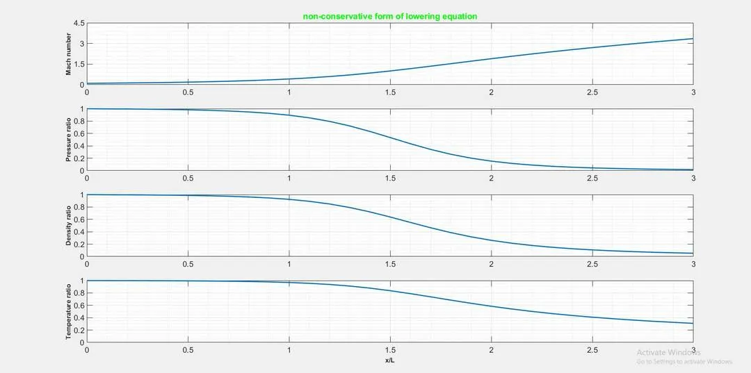
Figure 2:
x/L MACH number P/Po rho/rho0 T/To
| Non-cons | cons | Non-cons | cons | Non-cons | cons | Non-cons | cons | Non-cons | cons |
| 0 | 0 | 0.098782 | 0.098348 | 1 | 1 | 1 | 1 | 1 | 1 |
| 0.5 | 0.5 | 0.18703 | 0.18564 | 0.98232 | 0.98288 | 0.98734 | 0.98769 | 0.99492 | 0.99513 |
| 1 | 1 | 0.41552 | 0.41592 | 0.89547 | 0.89377 | 0.92414 | 0.92288 | 0.96896 | 0.96846 |
| 1.5 | 1.5 | 0.99937 | 0.98173 | 0.53424 | 0.54635 | 0.63869 | 0.65039 | 0.83646 | 0.84005 |
| 2 | 2 | 1.8901 | 1.9081 | 0.15316 | 0.15316 | 0.26184 | 0.25967 | 0.58495 | 0.57992 |
| 2.5 | 2.5 | 2.6963 | 2.7149 | 0.043785 | 0.043785 | 0.10721 | 0.10582 | 0.4084 | 0.40503 |
| 3 | 3 | 3.3532 | 3.367 | 0.016295 | 0.016295 | 0.052857 | 0.052717 | 0.30827 | 0.30549 |
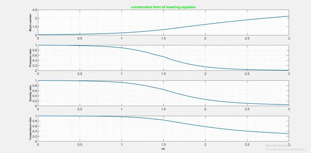
From the above plot and data we can notice that as the mach number increases flow reaches from subsonic to supersonic regime the primitve variables presure,density and temperature shows declivity after the sonic region (mach=1)till the exit of the nozzle.Although these results are almost identical to the analytical solution results validated from the CFD book by John D Anderson.
Figure(3):
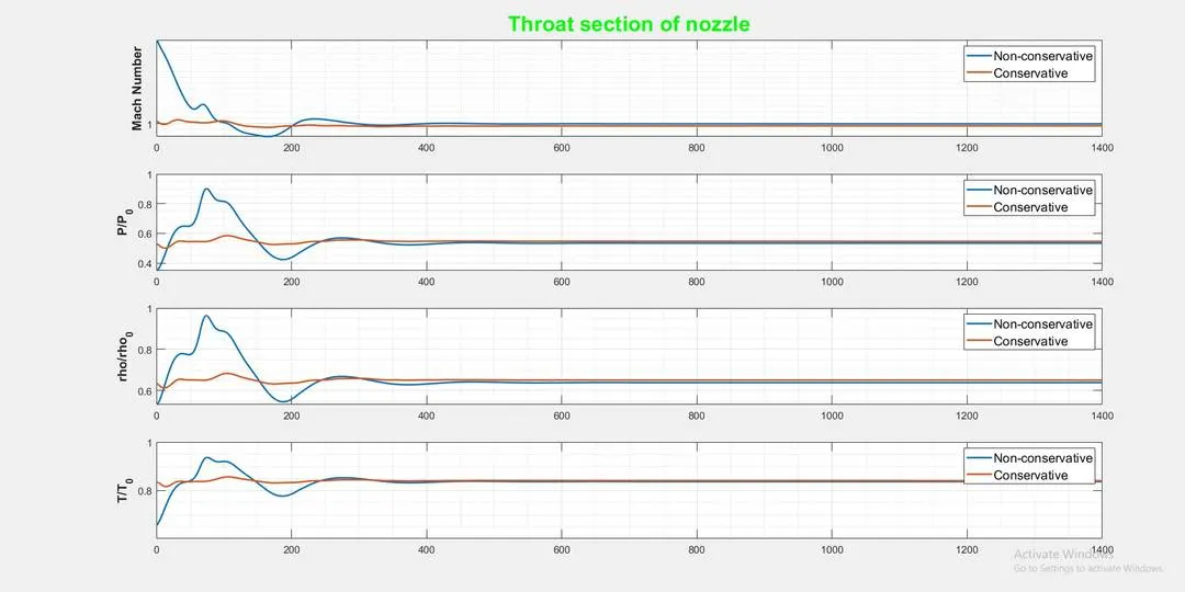
From the above plot for variation of different primitive variables w.r.t time steps,we can see that the conservative form,which we used the modified initial conditions,converges to the steady state faster than the non-conservative form.
Figure(4):
Figure(5):
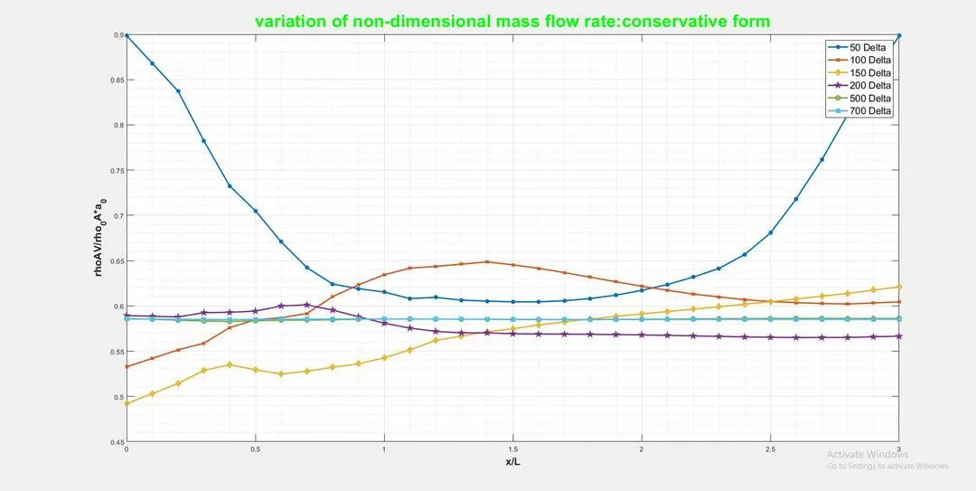
Figure(6):
Figure(7):
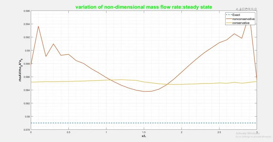
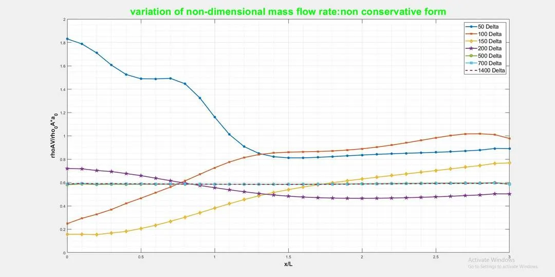
In the above plot,we compare the steady state variations of mass flow obtained with the non-conservative and conservative forms of the governing equations.Here we see that the steady state mass flow distribution predicted by the conservative form of the equations is much more satisfactory than that obtained from the non-conservative form ,on two accounts.
1.The conservative form gives a distribution i.e much closer to being a constant.In contrast,the non-conservative results have a sizeable variation with some oscillations at both the inflow and outflow boundary of course on a practical basis,these variations are not apparent and the mass flow essentially appears to be constant.
2.The steady state mass flow results obtained with the conservative form are,on the whole,much closer to the exact analytical solution.(rho'A'V'=0.579).
| Grid dependency test | rho/rho0 | T/To | P/Po | M |
| exact analytical solution | 0.634 | 0.833 | 0.528 | 1.00 |
| non-conservative form 31 grid points | 0.6387 | 0.8365 | 0.5342 | 0.9994 |
| conservative grid points 31 grid points | 0.6504 | 0.8401 | 0.5465 | 0.9817 |
| non-conservative form 61 grid points | 0.6376 | 0.8354 | 0.5326 | 0.9997 |
| conservative form 61 grid points | 0.6382 | 0.8352 | 0.5330 | 0.9993 |
The above discussion does not necessarily establish a definite superiority of the conservative form results over the non-conservative form result,let us look at the primitive variables in particular density,temperature ,pressure and mach number at nozzle throat as tabulated in the above table.By doubling the number of grid points the steady stae numerical results are slighlty closer to the exact,analytical values.for all the particular purposes we have grid independence with 31 grid points suffice to produce the steady state results .
The time taken for non-conservative form 31 grid points is 0.0755 sec and for 61 grid points =0.1014 sec.
The time taken for conservative form 31 grid points is 0.1130 sec and for 61 grid points =0.1478 sec.