Shock tube simulation project

Aim:-

• Setup the transient simulation for the shock tube.
• plot the Pressure and temperature history in the entire domain - Explain the result
• Plot the Cell count as the function of time.
• Show the generated mesh using paraview.
• create the species and velocity shock development animation.

Objective:-

• Import the geometry and provide 2 regions of different species with different pressure.
• Assign those regions to the boundary conditions.
• Setup the Transient type of simulation to observe the data with respect to time.
• Set event to set the time of open and close relation between two regions.
• Set AMR Adaptive Mesh Refinement for the species.
• Export all the preprocessed data for simulation.
• Post Process the velocity, pressure, and temperature data in Paraview.
• Create the animation of Adaptive mesh refinement in the Paraview.
• Also, create the animation of velocity, pressure, and temperature contour change with respect to time.

Shock Tube:-

• The shock tube is an instrument used to replicate and direct blast waves at a sensor or a model to simulate actual explosions and their effects, usually on a smaller scale.
• It is a device used to study transient aerodynamic phenomena under a wide range of temperatures and pressures for a variety of gases. It has been studied extensively by researchers from the start of the last century and has effectively served the developments of the supersonic and hypersonic flights and a range of transient devices, such as pulse-jet engines and a special supercharger called Comprex.
• A shock tube in its simplest form is a long tube with closed ends separated into two sections, namely, the driver section and the driven section, usually by a diaphragm.

Boundary Definition:-

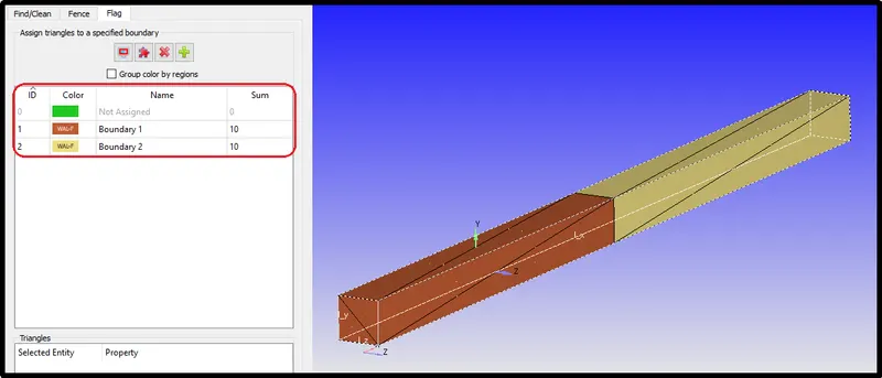
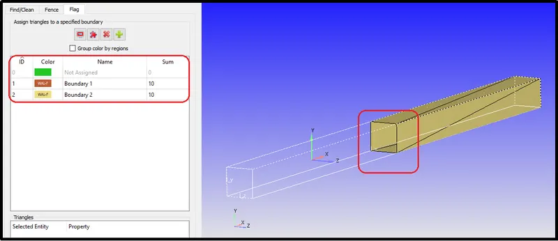
Set the two boundaries - boundary1, and boundary2 respectively.

Make Sure that there aren't any surfaces near the connection of those two boundaries.

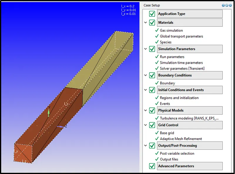
Simulation Setup/ Case setup:-

Application type:-

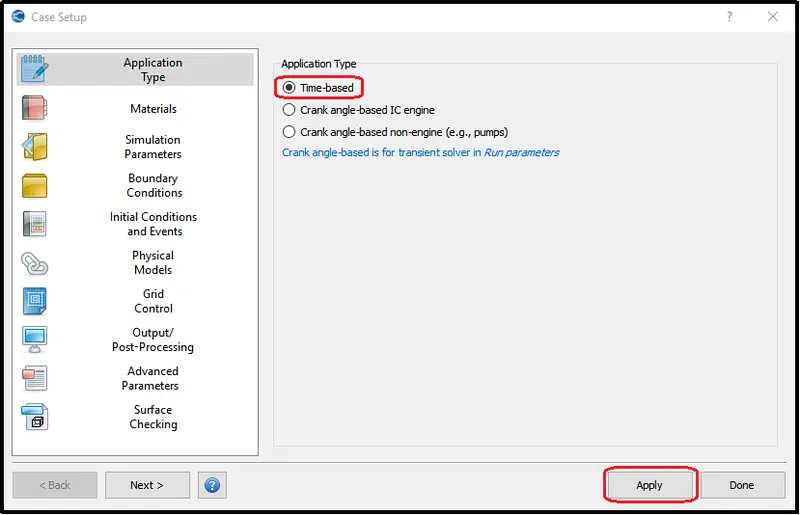
To begin with the transient state simulation in the 'Application Type" the "Time-based" must be selected and then, click apply and done.

Species:-

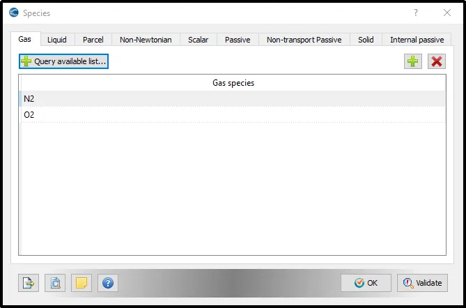
Mention all the species that going to be used in the simulation. In this particular case, N2 and O2, these two species were used.

Simulation Parameters:-

Run Parameters:-

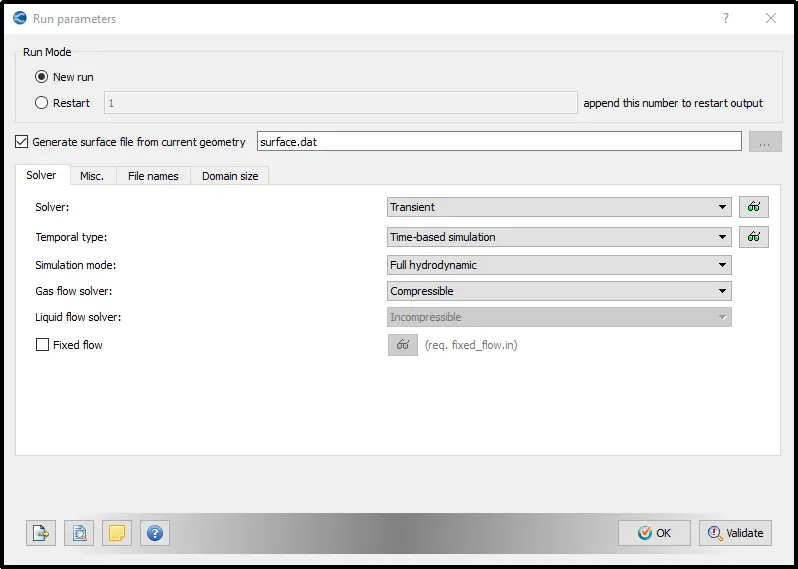
In the run parameter, we get to decide that either, we want steady-state simulation or Transient state simulation, so for the current simulation, the transient solver type was selected. This simulation involves the throttle movement which involves the changes in meshing while creating movement. To run this operation smoothly "NO hydrodynamic solver (for testing setup only)" option was chosen.

And, finally, as we are using air as a fluid that is compressible in nature so gas flow solver is set as compressible.

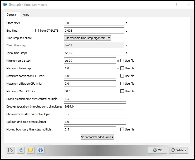
Simulation Time Parameters:-

Fluid Regions:-

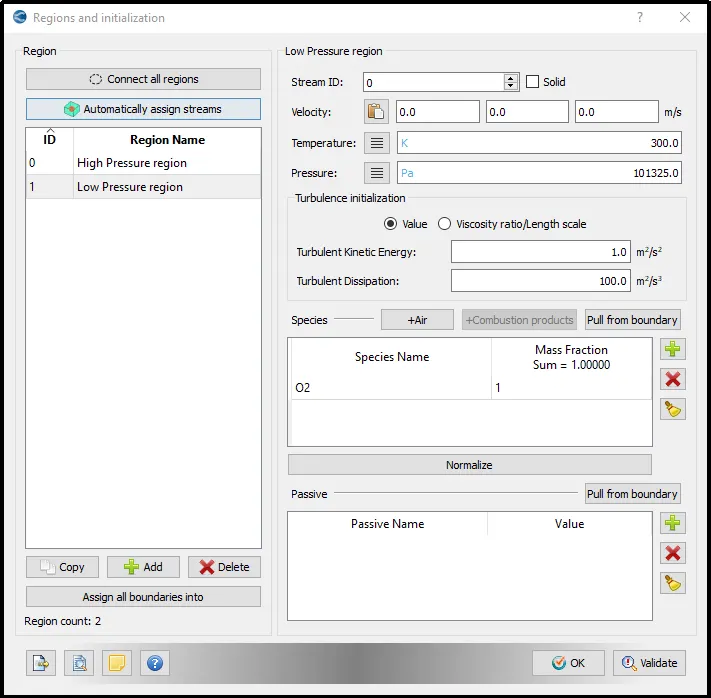
Especially, in this case, we need two regions - one is High-Pressure Region and another is a Low-pressure region.

For the High-pressure region, the pressure was set to 600000Pa.

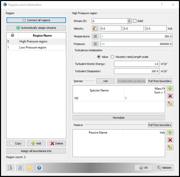
And, for the Low-Pressure region, we are considering atmospheric pressure.

Events:-

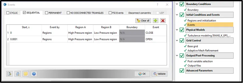
• Here, we are setting two events to define the boundary between two regions which can be open and closed by a defined time.
• So, for 0 to 0.0001 seconds the event will be closed, which means there will be no interaction between two boundaries.
• And, after, `0.0001^(th)` second, the boundary will open and both species will interact with each other.

Boundary Condition:-

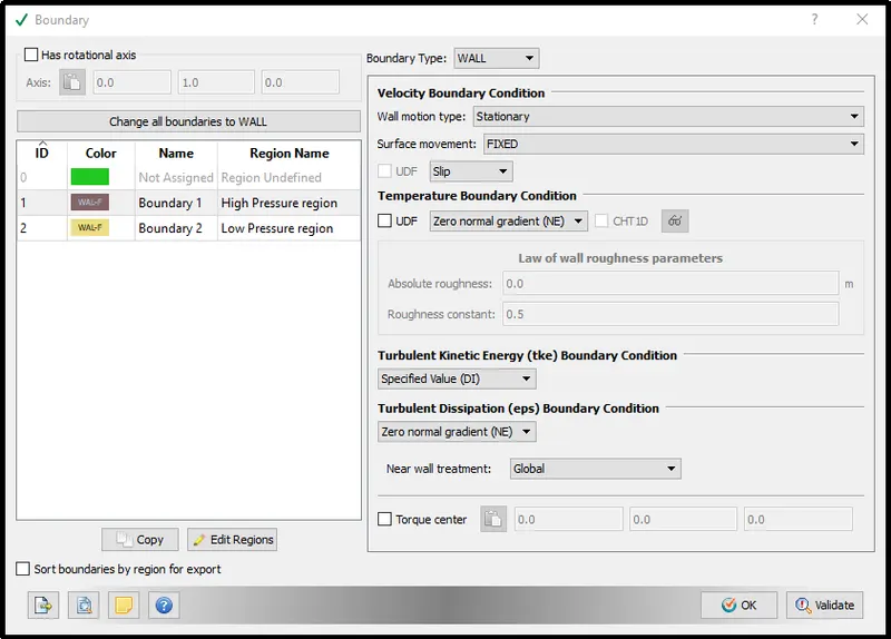
For all the faces of both boundary slip type condition was selected, which means there will be no friction between the fluid and the surfaces.

Turbulence model:-

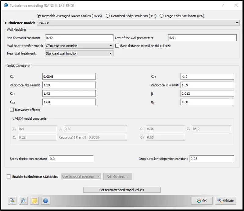
Here, the turbulence model was used as RNG K-epsilon. because because of obstacle or throttle valve the laminar stream converted into turbulent.

Meshing Parameters:-

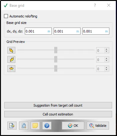
The grid size of 0.001m was given to all the directions.

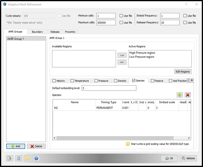
Adaptive Mesh refinement was considered for the species. In this setup, the mesh gets refine as per the changes in species interaction.

AMR Effect on the mixing of species in Shock Tube:-

Output/Post-processing:-

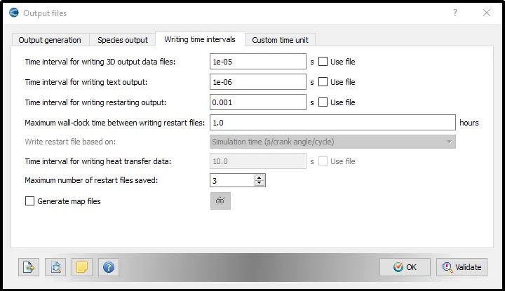
• To get 3D output Time interval for writing 3D output was set to 1e-05 sec means we are going to get 1 3D output after 1e-05 sec of the time step.
• The same calculation was used to get a time interval for text output data and a Time interval for waiting for restarting output files.

Export Input files:-

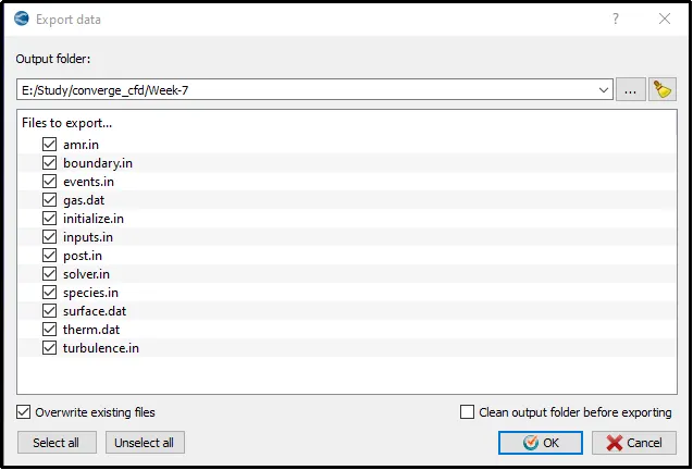
Using file -> Export -> Export Input files all the input files were exported to the simulation folder.

Results:-

Variation in Pressure and Temperature Contours with respect to time:-

Species Pressure Plot:-

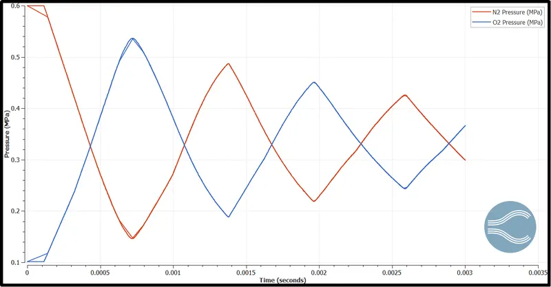
• In the pressure plot, we can notice the sum of pressure of both species remains constant throughout the simulation time. The pressure just passes from one gas to another which creates fluctuations in the shock tube.
• Another thing to notice, with time the fluctuations in the pressure of both systems stabilizing.

Species Temperature Plot:-

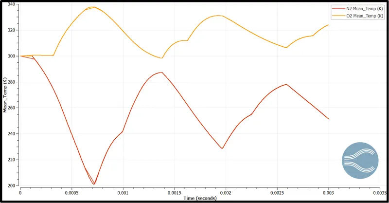
• In shock tube simulation the low-pressure gas is always the test species.
• when the diaphragm suddenly opens, which produces a series of compression waves, so that they quickly coalesce into a shock wave propagating into the low-pressure gas.
• The shock wave increases the temperature and pressure of the low-pressure gas adiabatically when sweeping through at shockwave velocity and also induces a fluid flow in the same direction but with a much slower velocity.
• Simultaneously, a fan of rarefaction (expansion) waves travels back into the high-pressure gas, decreasing its pressure and temperature.
• The interface separating low and high-pressure gases is referred to as the contact surface, which travels at the same velocity as the induced fluid flow between the shock and expansion wave.

Cell count as a function of time:-

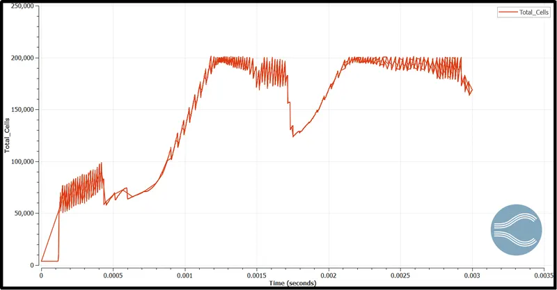
As we, set the AMR parameter for species, so for the species interaction region simulation refining the mesh size. As time passing both gases are mixing which means their interaction also increasing and so that the number of cells is increasing with time till the particular time. Then we can notice one sudden decline and rise of cell count because of the shock traveling through the shock tube.

Variation in Species and Velocity contours with respect to time:-

• In shock wave simulation, the driven (low-pressure) section of the shock tube is filled with the test gas mixture, in this case, O2.
• The driver section is overpressured with gas, often helium or a helium mixture, but in this case, N2 was used.
• The compressed gas fille in the tube until the diaphragm bursts. In the current simulation, we are using events for the opening of the diaphragm.
• An incident shock wave quickly forms and travels rapidly ahead of the driver gas into the driven section, increasing the temperature and pressure of the test gas, O2, behind it.
• On reaching the end wall of the shock tube, this incident shock wave reflects from the wall and propagates back toward the driver section, stagnating and further compressing and heating the test gas to its initial pre-reaction temperature and pressure.

Conclusion:-

• In a Shock tube, High-pressure driver gas expands upon the diaphragm opening, creating a shock wave.
• Test gas is instantaneously compressed and heated to combustion temperatures by the incident and reflected shocks.
• High-temperature experiments monitored near end wall
• shock tube has numerous practical applications such as the study of high-pressure, high-temperature chemistry, the design of supersonic vehicles and high power lasers, etc.
• Another very important application of a shock tube is its use in validating computational fluid dynamics codes.

References:-

[1] Shock tube - https://en.wikipedia.org/wiki/Shock_tube

[2] Shock tube techniques for kinetic target data to improve reaction models - https://www.sciencedirect.com/science/article/abs/pii/B9780444640871000036

[3] Screw pulsation generation and control: a shock tube mechanism - https://www.sciencedirect.com/science/article/pii/B9781782421696500097