Week 7: Shock tube simulation project
AIM: To Setup a transient shock tube simulation, to Plot the pressure and temperature history in the entire domain and to Plot the cell count as a function of time
Theoritical Background:
Shock Tube
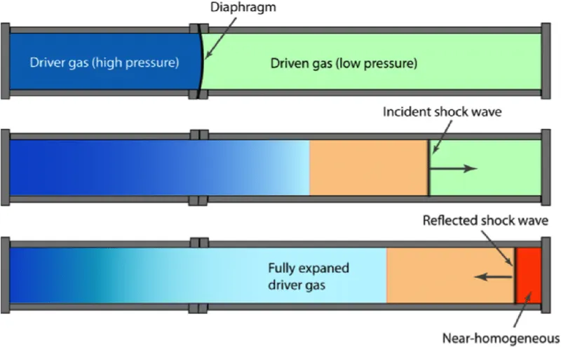
The shock tube is an instrument used to replicate and direct blast waves at a sensor or a model in order to simulate actual explosions and their effects, usually on a smaller scale. Shock tubes can also be used to study aerodynamic flow under a wide range of temperatures and pressures that are difficult to obtain in other types of testing facilities. Shock tubes are also used to investigate compressible flow phenomena and gas phase combustion reactions.
A shock wave inside a shock tube may be generated by a small explosion (blast-driven) or by the buildup of high pressures which cause diaphragm(s) to burst and a shock wave to propagate down the shock tube.
A simple shock tube is a tube, rectangular or circular in cross-section, usually constructed of metal, in which a gas at low pressure and a gas at high pressure are separated using some form of diaphragm. The diaphragm suddenly bursts open under predetermined conditions to produce a wave propagating through the low pressure section. The shock that eventually forms increases the temperature and pressure of the test gas and induces a flow in the direction of the shock wave. Observations can be made in the flow behind the incident front or take advantage of the longer testing times and vastly enhanced pressures and temperatures behind the reflected wave.
Geometry:
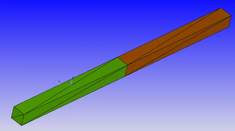

1] Materials:
Air as a mixture of Oxygen and Nitrogen is considered as the flow for the region
2] Simulation Parameters
Solver: Transient state density based solver
Simulation mode is Fully hydrodynamic and the gas flow solver is compressible
3] Simulation Time Parameters
Start Time = 0 seconds, End Time = 0.003 seconds, Initial time step = 1e-9 s, Minimum time step =1e-9 s
4] Regions and Initialization
2 regions are defined
High pressure region , velocity = [0,0,0] m/s, Stream ID = 0, Temperature = 300 K, Pressure = 600000 Pa
Low pressure region, velocity = [0,0,0] m/s, Stream ID = 0, Temperature = 300 K, Pressure = 101325 Pa
5] Boundary Conditions
We have to assign boundary conditions for different faces of Geometry as shown in the table below
Meshing
Base grid Mesh size , dx=dy=dz= 0.001m

Advance Mesh Refinement automatically refines the grid based upon flutuating and moving conditions. Advance Mesh Refinement is done to capture the flow properties in the shock region more accurately. The Mesh refinement takes place at N2-O2 interface and this mesh refinement keeps changing as the shock propogates back and forth

Pressure Contour
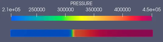
In the initial case setup we have mentioned 600000 Pa in the High Pressure region and 101325 Pa in the Low Pressure region. At Time Step = 20, diaphragm breaks, shock, slip surface and expansion waves are formed and propogate through the tube. Normal shock wave is formed which is propogates through the end of the tube until the end of the driven section. We observe that when the shock waves are created, expansion and retraction of the waves happens at the same instant. The shock wave produced is an oblique shock wave where the static properties such as Pressure, density and Temperature in the low pressure increase. The moment it hits the downstream end and get reflected their pressure value changes respectively and the flow pattern occurs till the shock intensity is decreased.
Temperature Contour
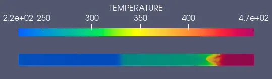
In the initial case setup we have mentioned 300 K for both High Pressure region and Low Pressure region. At Time Step = 20, diaphragm breaks and we can observe the cyclic motion of temperature variation across the cross section of the tube. Temperature also follows the same pattern as that of the pressure. The Temperature increases in the low pressure when the shock wave is generated after the diaphragm is ruptured. When the shock wave gets reflected the temperature in the low pressure region decreases
Mass Fraction of N2
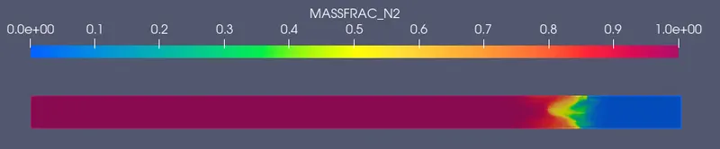
As the diaphragm breaks the N2 in the High pressure region pushers the O2 in the low Pressure region. The shock waves keep moving back and forth as the waves have different pressures. If the simulation is made to run for more time Pressure settels and converges to a value.
Velocity Contour

Pressure Plot
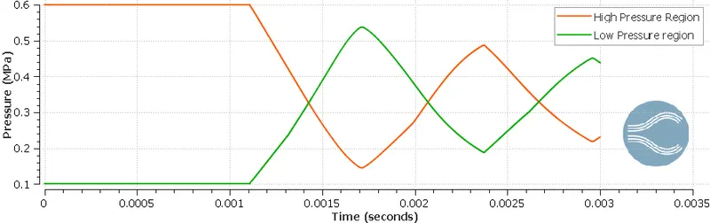
The High Pressure region is at 0.6 Mpa. As soon as the Diaphragm breaks both the Pressure regions(High and low ) pushes each other until reflected wave can occur. Shock wave generation leads to increase in Pressure in the low pressure region and decrease in pressure in the high pressure region. The pressure reaches a steady state value when the simulation is made to run for more time steps.
Temperature Plot
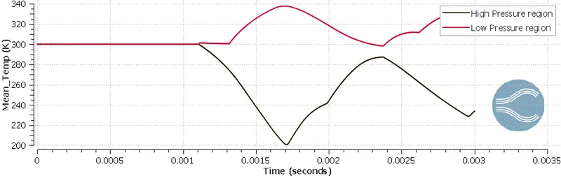
In the initial case setup we have mentioned 300 K for both High Pressure region and Low Pressure region. After the shock wave is generated the temperatures in both the regions vary cyclically. The temperature in the low pressure region vary between 300 K to 340 K. The Temperature in the High Pressure region vary between 200 K to 300K and reaches a steady state.
Cell Count Plot
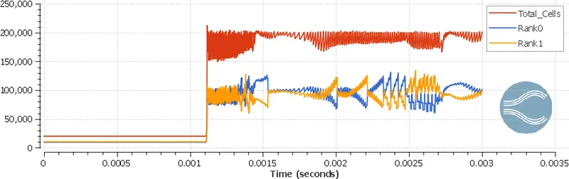
The Cell count is changing due to the adaptive mesh refinement depending upon the species that we have given. As the diaphragm breaks the N2 in the High pressure region pushers the O2 in the low Pressure region. N2 will enter the low pressure region and cause the mesh to become finer. The Mesh becomes finer as a result of which cell count will increase and it takes place until the equillibrium is obtained. Uniform pressure is obtained in the shock tube after both the gases diffused completely.