Week 7: Shock tube simulation project

AIM:

To Setup a transient shock tube simulation.

Objective:

• Plot the pressure and temperature history in the entire domain - Explain the result
• Plot the cell count as a function of time - Explain the result

Introduction:

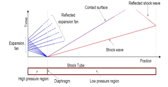
The shock tube is an instrument used to replicate and direct blast waves at a sensor or a model in order to simulate actual explosions and their effects, usually on a smaller scale. Shock tubes (and related impulse facilities such as shock tunnels, expansion tubes, and expansion tunnels) can also be used to study aerodynamic flow under a wide range of temperatures and pressures that are difficult to obtain in other types of testing facilities. Shock tubes are also used to investigate compressible flow phenomena and gas phase Combustion reactions. More recently, shock tubes have been used in biomedical research to study how biological specimens are affected by blast waves.

A shock wave inside a shock tube may be generated by a small explosion (blast-driven) or by the buildup of high pressures which cause diaphragm(s) to burst and a shock wave to propagate down the shock tube (compressed-gas driven).

Procedure:

Step:1

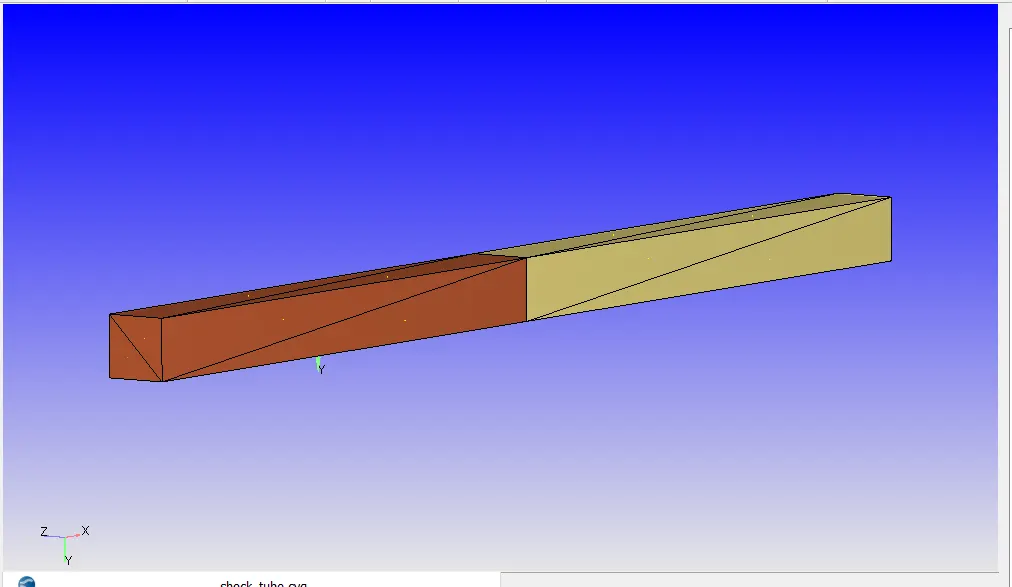
Import given geomentry

Step:2:

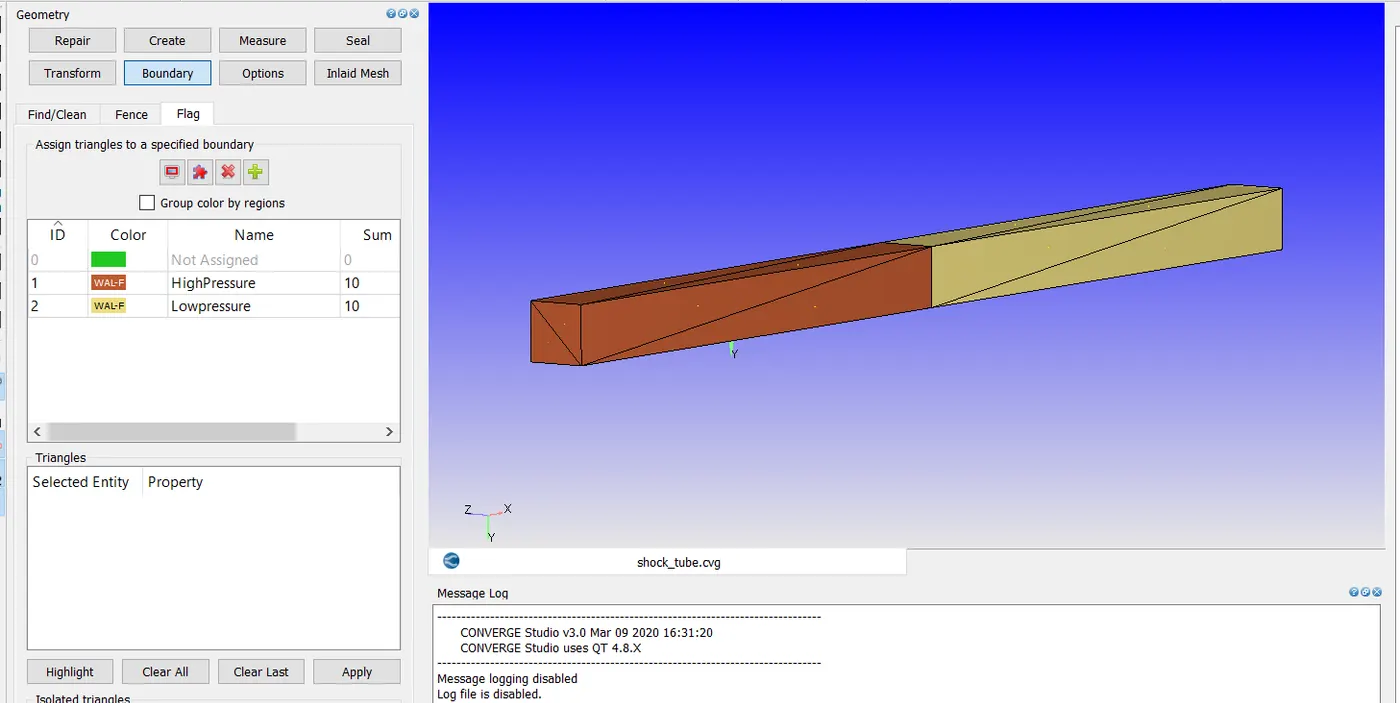
In this step, we take triangular structures and flag them together as boundaries which are marked with different colours. This is done so that the boundary conditions can be assigned to each triangular structure.

Giving boundaries by selecting the sides which can help with other steps for simulation.

Once the boundaries have been flagged, we assign the different boundary conditions for the flow to take place within the geometry.

Step:3:

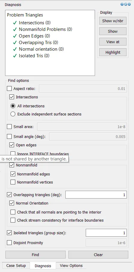
Check whether there is any errors by using diagnosis tool as shown below.

Step:4:

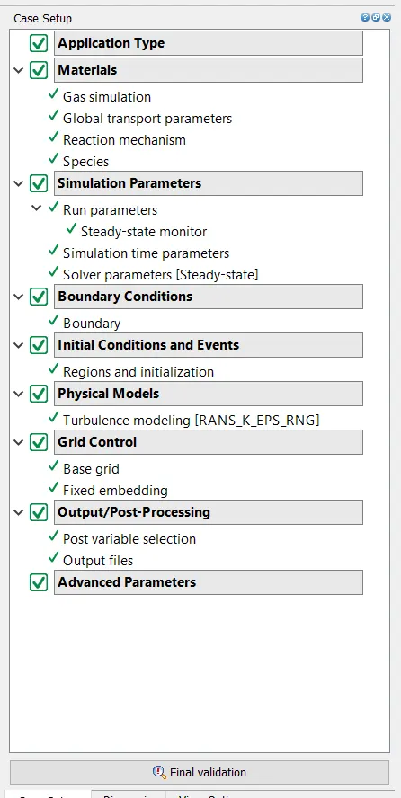
These are the following steps for setting up simulation for Backward facing step.

Step:5:

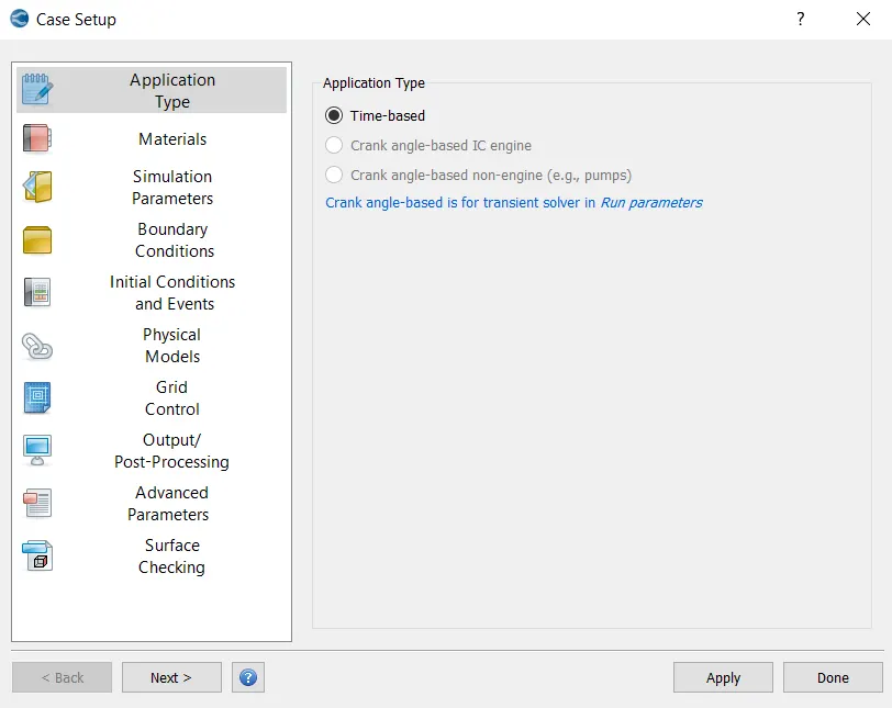
Select the application type time based for steady state simulation.

Step:6:

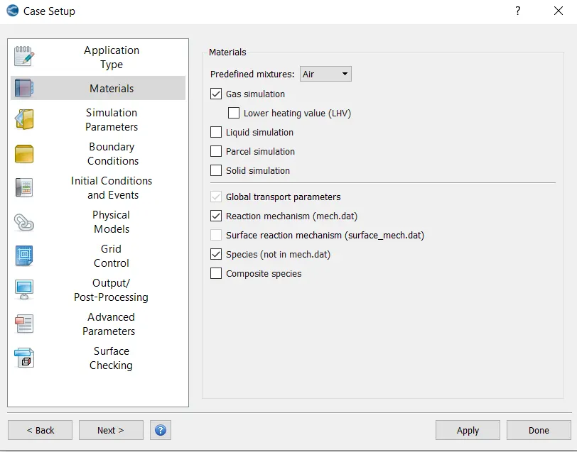
Select the material type for the flow through geomentry .here Air is the material taken.

Step:7

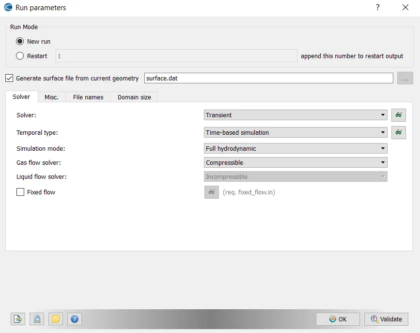
Select transient for the simulation.

Step:8:

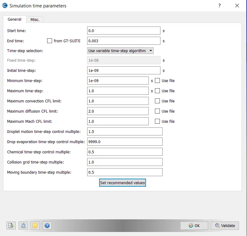
Here we can define the start and end time of simulation

and also the initial and minimum time step.

Step:9:

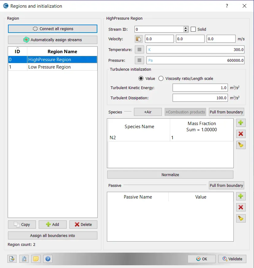
The boundaries are to bounded to a region for the transient simulation.so that Both regions are created with the species of air.

High Pressure Region:

Here the pressure is specified as 6 bar.

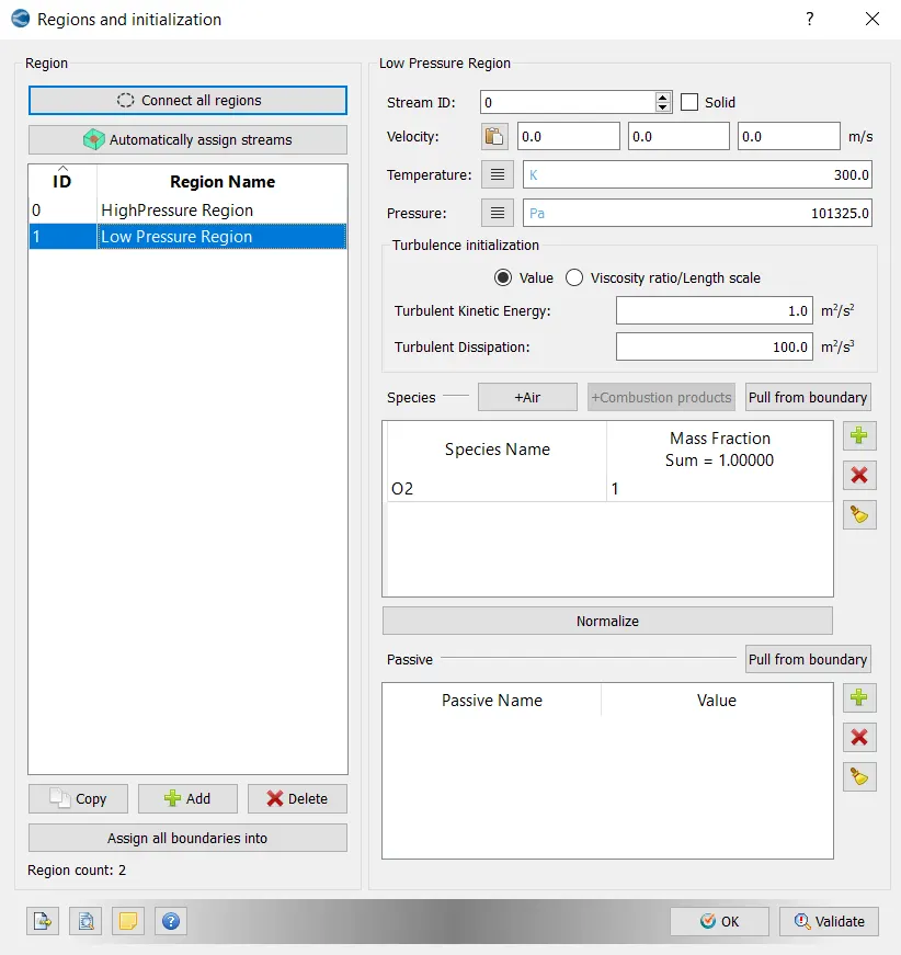
Low Pressure Region:

Default specification

Step:10:

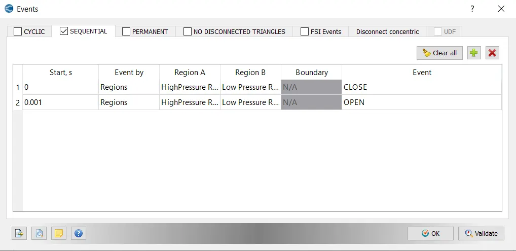
Creating events:

Here the events are created to open and close of the Diaphragm .

Step:11:

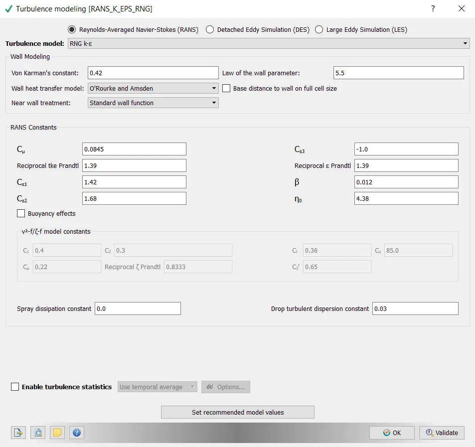
Here select the turbulance model that can be used for simulation.

Step:12:

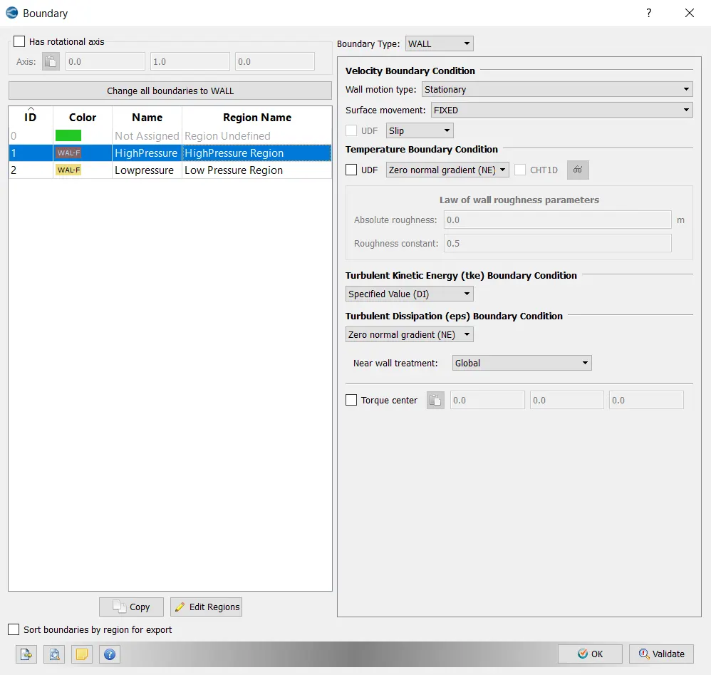
In here the boundary conditions are given to the Both specified regions .

both High and low pressure regions are specified as slip walls.

Step:13:

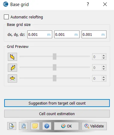
The basic mesh size of the Geomentry is specified here.

Step:14:

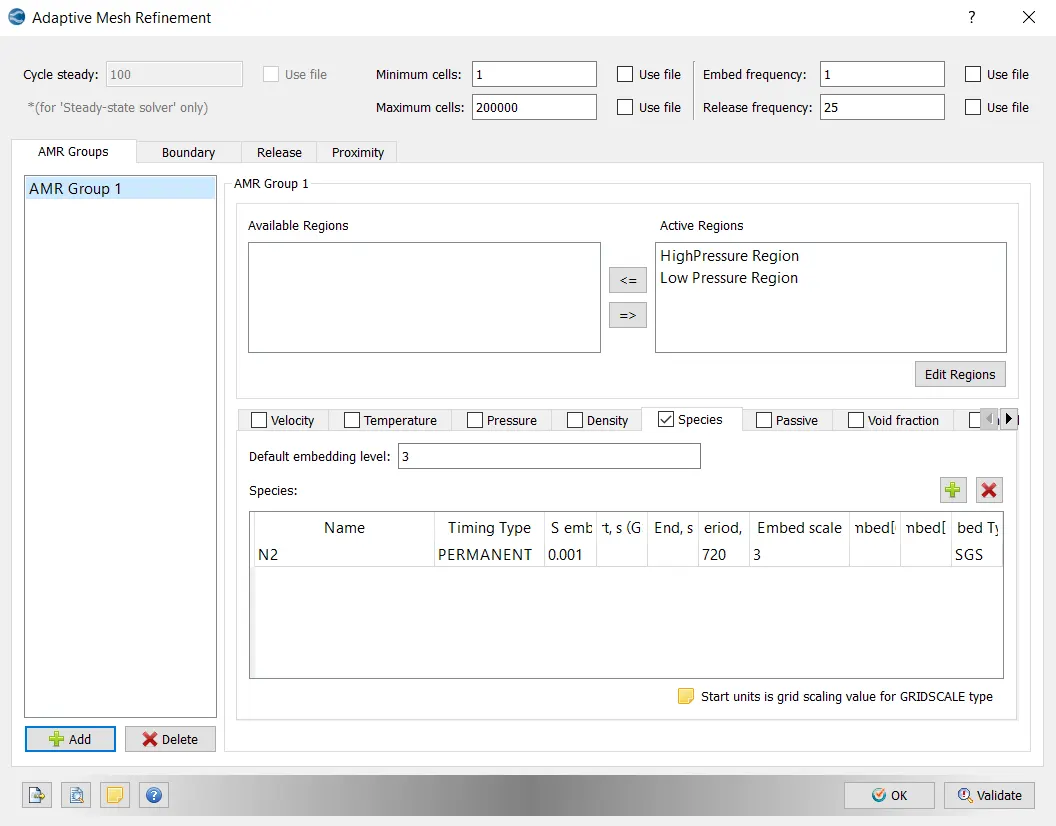
Adaptive mesh refinement where the regions are specfied to active regions and species time and scale are specified.

Step:15:

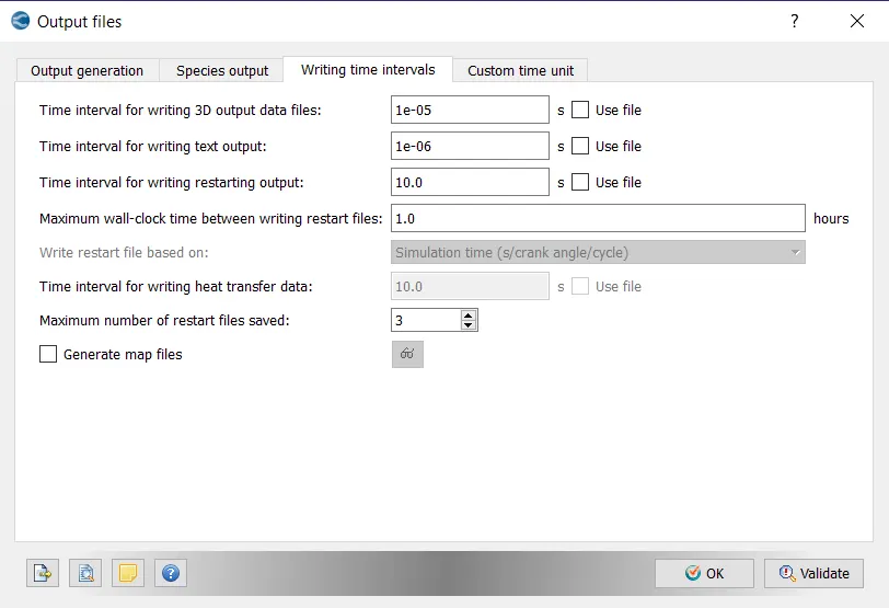
Writting the output files intervals.

Step:16:

Finally the specified case setup file are exported to folder and run simulation.

The simulation for number of cycles are run in cygwin command window.

Step:17:

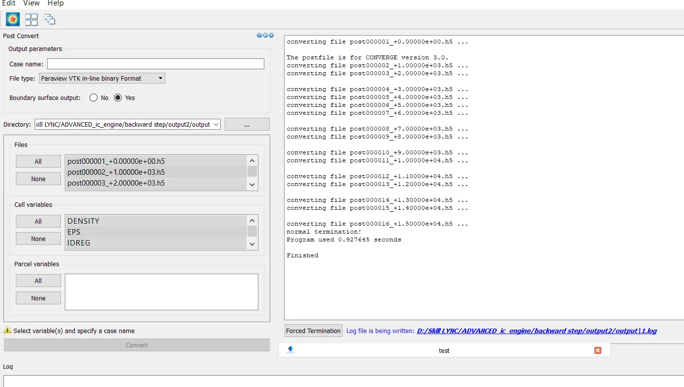
Post convert the files that is simulated in cygwin command window and file name is given .

Step:18:

Software used: ParaView As the simulation is binary files called “post” files are generated inside the output folder. These files have an extension *.out. Now these files are written by CONVERGE. These files contain information regarding the 3D flow field. We use a special software called ParaView that can read this flow information. However, before ParaView can do this, the files have to be converted to a form that ParaView can understand. This is done using a tool called post convert. After the conversion, we load the files into ParaView.

Results:

Animations:

velocity in shocktube:

pressure in shocktube:

AS the pressure between the two regions is 5 bar. the mixing occures the pressure difference occurs in both regions.As the high pressure gas starts mixing with the low presure gas, thus it leads to formations of shock waves due to the difference in pressure. These shock waves travel to and fro in the domain due to reflection of walls.

The pressure of N2 gets dropped due to expansion and the pressure of o2 gets increases due to compression of gas.

Above animation we can clearly see that the waves travelling from higher presure region to lower pressure region when it reaches the dead end it reflects back and travel in the opposite direction.

Temperature in Shock tube:

From the above animation in the higher pressure region the temperature is constant at the initial stages after the opening of diaphragm The temperature decreases due to pressure decrease.

we can see the fluctuvations in shock waves as it moves front and back in the domain.when it moves backwarsds the temperature is high region starts increasing and the low regions starts decreasing simultaniously.

mass fraction of N2:

From the animation we can observe that the diaphragm breaks the N2 gas is entered into the low pressure region and as soon as it reaches the end, the reflected shock waves pushes back in the reverse direction and reflected back from the other end of the tube that pushes the N2 gas in the direction of other end. this process continues till the shock waves are declined.

The Generation of Mesh:

The graph that shows the total cell counts:

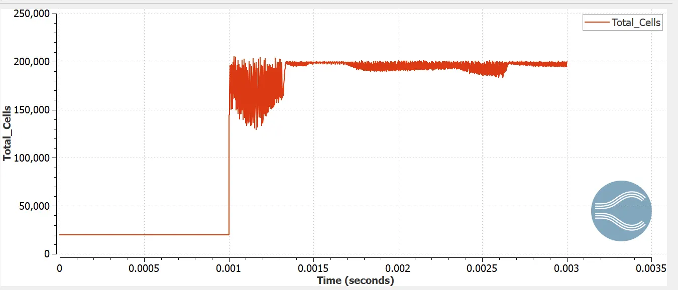
The total cells in the domain can be varied due to burst of diaphragm amd also we used the Amr technique for this so we can observer the increase in the number of cells in some regions.

Conclusion:

Sucessfully demonstrated the transient shock tube simulation and aslo observed how the species is mixing in the shock tube.

AS the pressure between the two regions is 5 bar. the mixing occures the pressure difference occurs in both regions.As the high pressure gas starts mixing with the low presure gas, thus it leads to formations of shock waves due to the difference in pressure. These shock waves travel to and fro in the domain due to reflection of walls.