Week 7: Shock tube simulation project

• Setup a transient shock tube simulation
• Plot the pressure and temperature history in the entire domain - Explain the result
• Plot the cell count as a function of time - Explain the result

It is expected to show the mesh generation using PARAVIEW.

Also create an animation and upload it on You tube and provide the You tube link for an animaion in your report.

Solution

Aim

•  To run a transient shocktube simulation using CONVERGE CFD.
•  Shock tubes are devices used to replicate exposions and their effects on an object in small scales by subjecting the test object to direct blast waves.
• The blast waves are usually generated by the buildup of high pressures which cause diaphragm(s) to burst and a shock wave to propagate down the shock tube.

Objective: 

• Setup a transient shock tube simulation
• Plot the pressure and temperature history in the entire domain - Explain the result
• Plot the cell count as a function of time - Explain the result

SOFTWARES USED:

• Converge Studio v3.0
• Windows CMD and CYGWIN
• Paraview

Introduction:

• The shock tube is an instrument used to replicate and direct blast waves at a sensor or a model in order to simulate actual explosions and their effects, usually on a smaller scale.
• A simple shock tube is a tube, rectangular or circular in cross-section, usually constructed of metal, in which a gas at low pressure and a gas at high pressure are separated using some form of diaphragm. See, for instance, texts by Soloukhin, Gaydon and Hurle, and Bradley.

Shocktube:

• The Shocktube is a tube made out of metal that consists of two chambers separated by a diaphragm. The two chambers consist of two gases with a large pressure ratio. The gas of higher pressure is called the Driver Gas and the other one is called the driven gas. The chambers are also termed Driver and Driven.
• The diaphragm is builtin with a puncturing mechanism that breaks the diaphragm under predetermined conditions. 
• The breaking of the diaphragm causes a drastic onset of compression pressure waves towards the low-pressure region due owing to a sudden pressure difference. The leading pressure wave is called the Shockwave. This shockwave is followed by a series of more pressure waves which raises the temperature and pressure of the driven gas. Simultaneously, a rarefaction wave formed in the opposite direction of the shockwave which travels towards the driver chamber. 
• One of the main applications of shock tubes includes the study of the chemical kinetics of fuels. The chambers of the shock tube would be filled with an Air-Fuel mixture; As the shock propagates, the pressure and temperature rise. When the temperature attains the auto-ignition temperature, the fuel ignites. Hence this can also be used to find the auto-ignition delay of the fuel. 

Regions and Events:

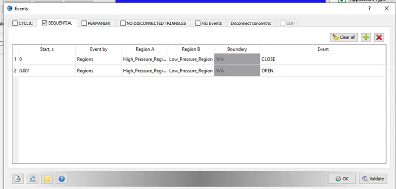
• In Converge, a 'Region' is a collection of boundaries used to delineate different areas in a geometry. Let us take the example of the shock tube itself. In the shock tube, there exists a High-pressure(HP) region and a Low-pressure(LP) region. These two must be separated initially which is taken care of by regions.
• Events is a feature that engages and disengages two boundaries. In a real shock tube, there is a diaphragm that prevents mixing between the two chambers. To incorporate this effect in the simulation, a region is added, and using events, the disengagement of the region is simulated. At time t>0, the initial engagement is disengaged and the pressure difference creates a shockwave.
• Internally, the Converge solver creates a temporary obstruction using triangles to from regions. These temporary triangles are called Disconnect Triangles. There are two types of disconnect triangles- Single Loop and Concentric.

In the shocktube simulation, single-loop disconnect triangles are used, as the interface region between both the regions are of the same dimensions;

 Steps Required for this simulation

• Geometry
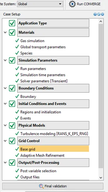
• Case setup
• Run the simulation in Cygwin
• Post process results in Para view

Geometry:

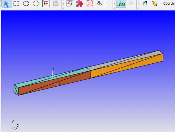
Import the STL file into the converge

Check the normal

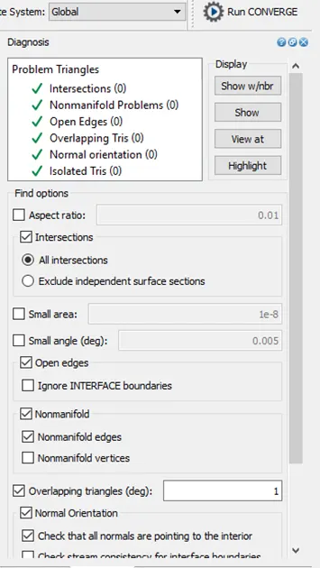
Check diagnosis if whether there is any fault in geometry and correct them

 

 Diagnosis Dock

 

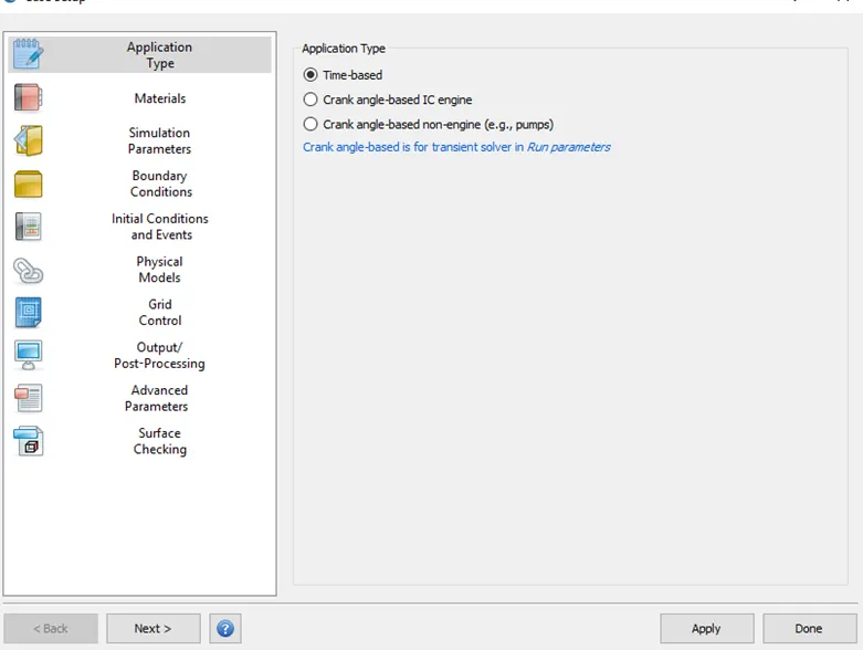
Case setup

Application Type

Application type: Time based- General flow

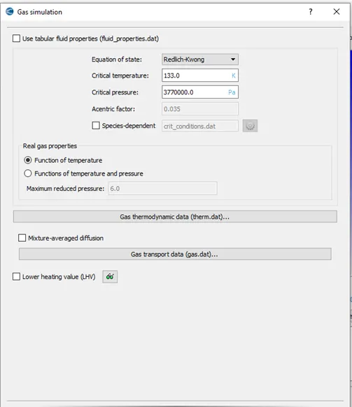
Materials : Air

 

Gas Simulation

 

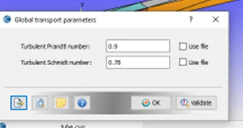
Global Transport parameters

 

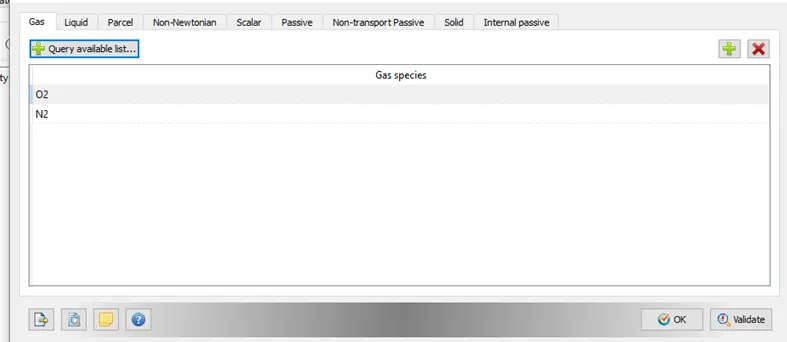
 Species

 

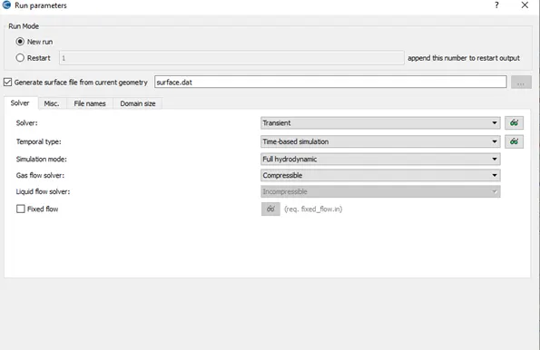
Run parameters

Slover: Transient

 

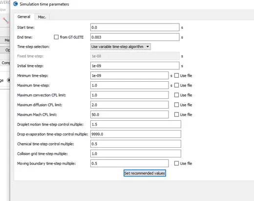
Simulation Parameters

Start time -0

End time:0.003 s

Initial time steps: 1e-09 s

Minimum Time Steps:1e-09 s

Maximum time steps: 1 s

 

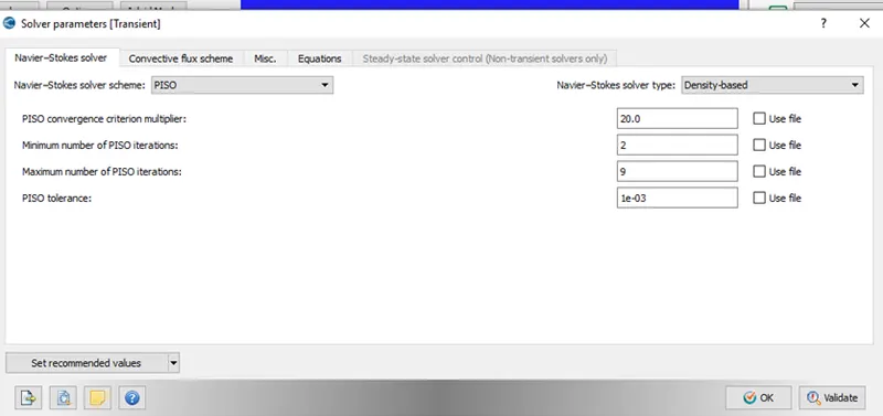
Slover parameters

Slover: Density Based Transient State Slover

 

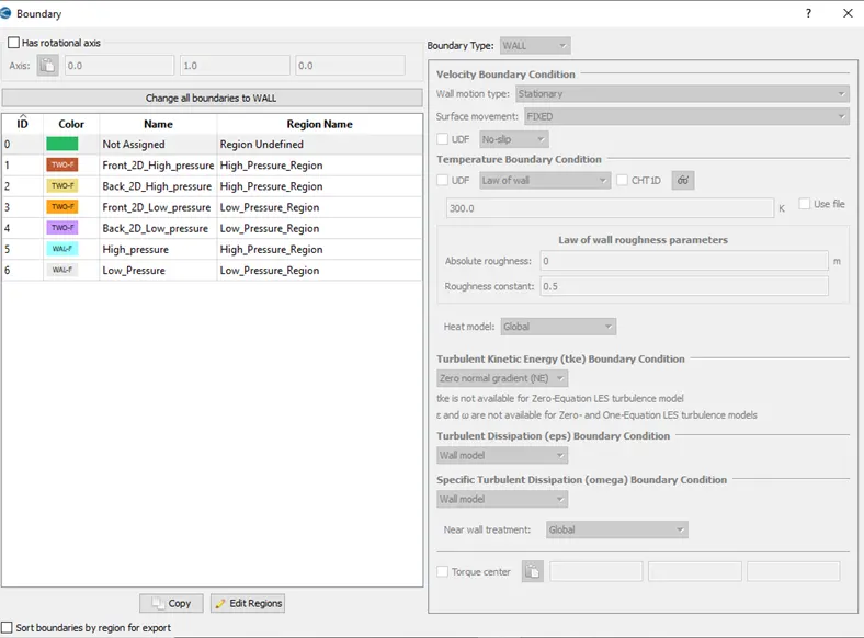
Boundary Condition

• High pressure Wall – slip

Temperature: 300 k

• Low pressure Wall – slip

                Temperature: 300 k

• Front – 2D for both region
• Back-2 D for both region

 

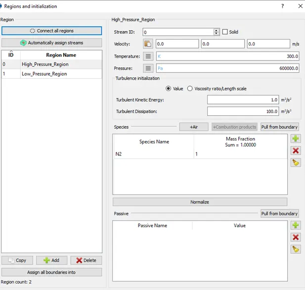
Region and initialization

High Pressure Region

• Region 0 – high pressur
• Pressure : 600000 pa
• Species N2 : 1

 

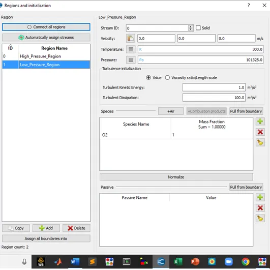
Low pressure region

• Region 1 – low pressure
• Pressure : 101325 pa
• Species O2 : 1

 

Events:

 

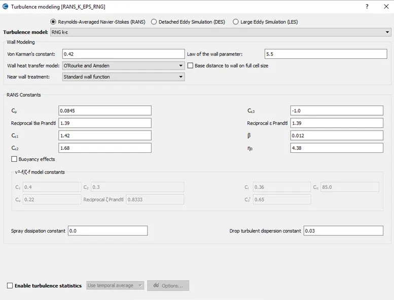
Turbulance Modelling

 

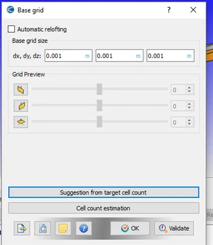
Base Grid

 

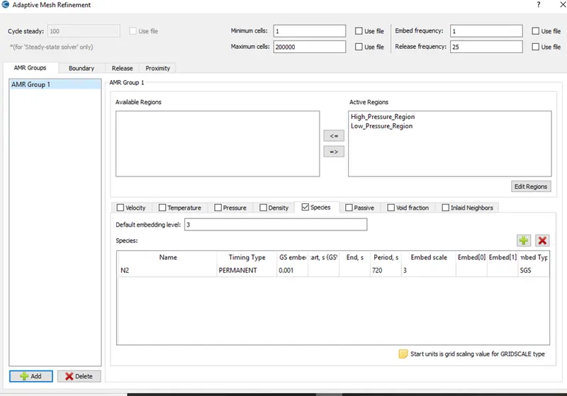
 Adaptive Mesh Refinement

 

 Final Validation

 

Mesh

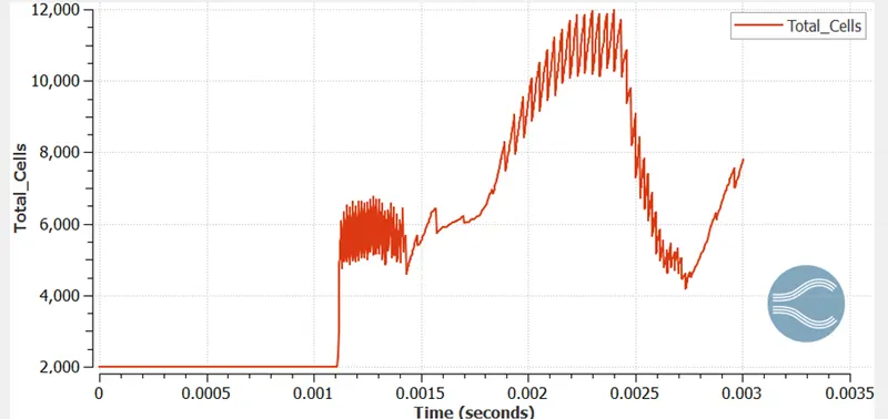
Total Cell Count:

Due to the Adaptive mesh refinement, it can be seen that the cells are changing with respect to time. We see that diaphragm has ruptured at 0.001 s the mesh size start changes. The refinement of cells is done according to SGS Criteria,

 

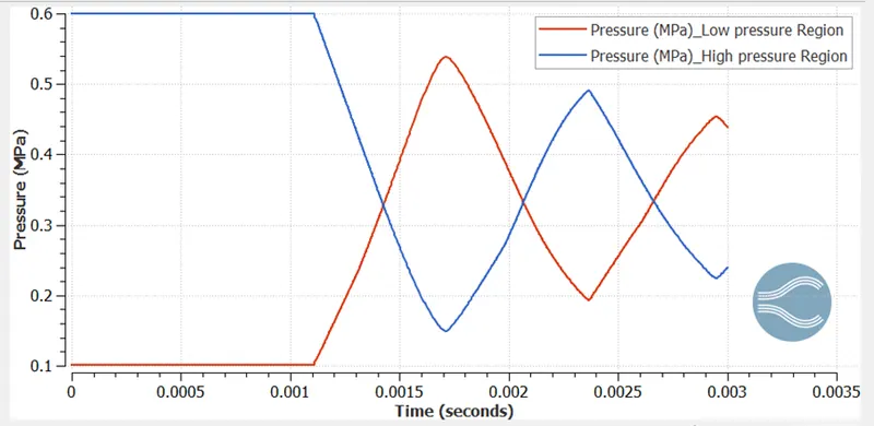
Pressure at Low pressure Region and high-pressure Region:

• Below graphs shows variation at high pressure region and low-pressure region.
• There is increase pressure in low pressure region and decreases pressure in High pressure region
• The pressure changes accordingly when the shock front is reflected back

 

 

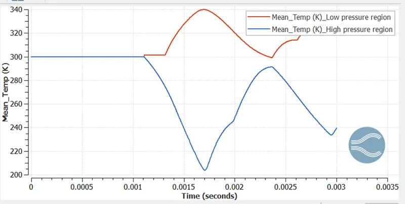
Mean Temperature at Low pressure Region and high-pressure Region

• Below graphs shows variation of mean temperature at high pressure region and low-pressure region.
• Temperature at low pressure region increases and Temperature at High pressure region decreases.
• Changes of temperature was seen with to & fro Movement of Shock

 

Pressure contour

Velocity Contour

Temperature Contour

Mass fraction of N2 across the tube: N2 from high pressure region produce shock and passes to the low pressure O2 region

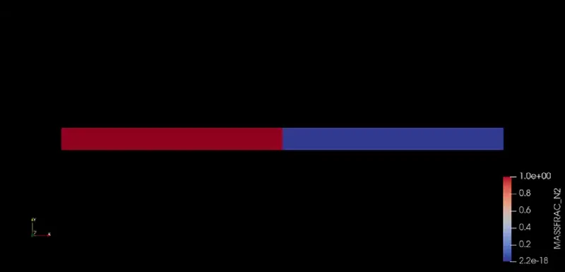
Animation Link : https://youtu.be/0he3az81zMY

velocity Magnitude

Animation Link : https://youtu.be/YIGiQm9E14o

Conclusion

• Simulation is run successfully for given shock tube problem
• There is increase pressure in low pressure region and decreases pressure in High pressure region
• The pressure changes accordingly when the shock front is reflected back
• We can easily conclude that cell count is function of time, AMR Phenomenon was studied