Week 7 - Auto ignition using Cantera

AIM:

• To determine Auto-ignition delay for methane combustion for the cases as shown:

1. For varying temperature from 950K to 1450K under constant pressure.
2. For varying pressure 1bar – 5bar under constant temperature.

• Finding the molar concentration of H2O, O2, OH

1. When temperature is 1000K and 5 bar.
2. When temperature is 500K and 5 bar.

Theory

A cantera reactor represents the simplest form of chemically reacting system. It corresponds to an extensive thermodynamic control volume, in which all the state variables are homogeneously distributed. The system in generally unsteady .i.e. all states are function of time. In particular, transient state changes are possible due to chemical reactions. Further, thermodynamic equilibrium is assumed o be present throughout the reactor at all instants of time.

There are different type’s reactors available in cantera as explained:

1. Expansion /Compression Work: By moving the walls of the reactor, the volume of the reactor can be changed.
2. Heat Transfer: Arbitrary heat transfer can be defined across the walls of the reactor.
3. Mass Transfer: The reactors can be made with different inlet and outlets allowing the mass transfer.
4. Surface Interaction: In this type influence of chemical reaction due to walls can be studied. This can also include mass transfer in between surface and fluids.

These interactions in cantera don’t always need to be constant but can be also be set as function of state or time. For instance heat transfer can be defined as the function of temperature difference between the reactor and the environment, or change in volume as a function of pressure.

In addition to single reactors multiple reactors can also be interconnected with the help of the reactor network. Each reactor in a network may be connected so that one reactor flow into another. Reactors can also be in contact to each other or the environment via walls that conduct heat or move to do work.

CASE I

For the first case the code is written in python using the cantera module to simulate the Methane combustion and obtain the ignition delay parameters for different pressure and temperature. The Auto ignition delay is defined as the time for which the temperature is raised by 400K with respect to the initial temperature.

For these simulation ideal gas reactors has been used for the study and corresponding reactor network.

1. For the temperature varying from 950K to 1450K while keeping the pressure constant. Here 5 equidistant temperature values are being considered for this case:

The python Code is shown below:

import matplotlib.pyplot as plt
import cantera as ct
import numpy as np


gas = ct.Solution('gri30.xml')
t_start = 950
t_end = 1450
P = 5*101325
#a = 0

sim_time = 5000

temp = np.linspace(t_start,t_end,5)
ignition_delay = []
for T in temp:
	gas.TPX = T, P, {'CH4':1, 'O2':2, 'N2':7.52}
	r = ct.IdealGasReactor(gas)
	sim = ct.ReactorNet([r])
	time = 0
	T_old = T
	a = 0

	states = ct.SolutionArray(gas, extra = ['t_ms','t'])

	for i in range(sim_time):
		time += 1e-4
		sim.advance(time)
		states.append(r.thermo.state, t_ms = time*1e3, t = time)
		T_new = states.T
		T_new = T_new[i]
		

		if ((T_new - T_old) >=400 and a==0):
			ignition_delay.append(time)
			a = a + 1
		
	plt.figure(1)
	plt.plot(states.t_ms, states.T)
plt.legend(['T_Start =' + str(P/101325) + '[K]' for T in temp])
plt.xlabel('Time [ms]')
plt.ylabel('Temperature [K]')
#plt.show()

plt.figure(2)
plt.plot(temp,ignition_delay,'-o')
plt.xlabel('Temperature [K]')
plt.ylabel('ignition_delay [ms]')
plt.show()

print('ignition_delay = ', ignition_delay)
print('Temperature = ', temp)

2. For the pressure varying from 1bar to 5bar while keeping the temperature constant. Here 5 equidistant pressure values are being considered for this case:

The python Code is shown below:

import matplotlib.pyplot as plt
import cantera as ct
import numpy as np


gas = ct.Solution('gri30.xml')
p_start = 1*101325
p_end = 5*101325
T = 1250
a = 0

sim_time = 5000

pressure = np.linspace(p_start,p_end,5)
ignition_delay = []
for P in pressure:
	gas.TPX = T, P, {'CH4':1, 'O2':2, 'N2':7.52}
	r = ct.IdealGasReactor(gas)
	sim = ct.ReactorNet([r])
	time = 0
	T_old = T
	a = 0

	states = ct.SolutionArray(gas, extra = ['t_ms','t'])

	for i in range(sim_time):
		time += 1e-4
		sim.advance(time)
		states.append(r.thermo.state, t_ms = time*1e3, t = time)
		T_new = states.T
		T_new = T_new[i]
		

		if ((T_new - T_old) >=400 and a==0):
			ignition_delay.append(time)
			a = a + 1
		
	plt.figure(1)
	plt.plot(states.t_ms, states.T)
plt.legend(['P_Start =' + str(P/101325) + '[bar]' for P in pressure])
plt.xlabel('Time [ms]')
plt.ylabel('Temperature [K]')
#plt.show()

plt.figure(2)
plt.plot(pressure,ignition_delay,'-o')
plt.xlabel('Pressure [Pa]')
plt.ylabel('ignition_delay [ms]')
plt.show()

print('ignition_delay = ', ignition_delay)
print('Pressure = ', pressure)

RESULTS

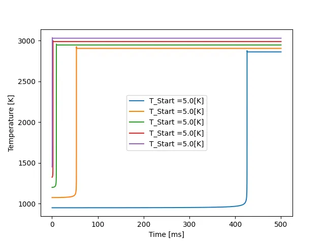
For temperature varying from 950K to 1450K under constant pressure.

Graph (Temperature (K) vs Times(ms)) can be seen below.

Graph (Temperature (K) vs Ignition Delay (ms)) can be seen below.

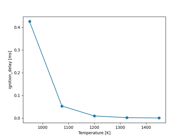
It can be clearly noted that ignition delay decreases with increase in temperature which means that ignition delay is sensitive to temperature.

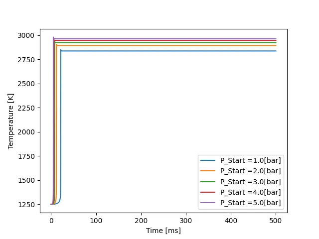
For Pressure varying from 1bar to 5bar under constant temperature.

Graph (Temperature (K) vs Times(ms)) can be seen below.

Graph (Temperature (K) vs Ignition Delay (ms)) can be seen below.

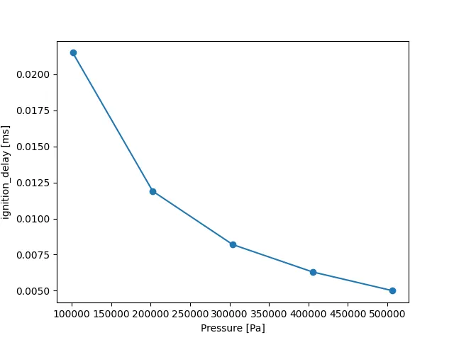
It can be clearly noted that ignition delay decreases with increase in pressure which means that ignition delay is sensitive to pressure. Further it can also be noted from the above plot that ignition delay is more sensitive to temperature than to pressure.

CASE II

For the second case we will find the molar concentration for H2O, OH, O2 for the conditions shown below:

1. When temperature was 1000K and the pressure is 5bar.
2. When temperature was 500K and the pressure is 5bar.

The code can be seen below for the temperature of 1000K and 5bar.

import matplotlib.pyplot as plt
import cantera as ct
import numpy as np


gas = ct.Solution('gri30.xml')

P = 5*101325
#a = 0

sim_time = 10*1000

temp = [500,1000]
ignition_delay = []
for T in temp:
	gas.TPX = T, P, {'CH4':1, 'O2':2, 'N2':7.52}
	r = ct.IdealGasReactor(gas)
	sim = ct.ReactorNet([r])
	time = 0
	T_old = T
	#a = 0

	states = ct.SolutionArray(gas, extra = ['t_ms','t'])

	for i in range(sim_time):
		time += 1e-3
		sim.advance(time)
		states.append(r.thermo.state, t_ms = time*1e3, t = time)
		

		
	plt.figure(1)
	plt.plot(states.t, states.X[:,gas.species_index('H2O')])
	plt.xlabel('Time [ms]')
	plt.ylabel('Species Concentration [H2O]')
	#plt.show()
	
	plt.figure(2)
	plt.plot(states.t, states.X[:,gas.species_index('O2')])
	plt.xlabel('Time [ms]')
	plt.ylabel('Species Concentration [O2]')

	plt.figure(3)
	plt.plot(states.t, states.X[:,gas.species_index('OH')])
	plt.xlabel('Time [ms]')
	plt.ylabel('Species Concentration [OH]')
	plt.show()

RESULTS:

CASE I:

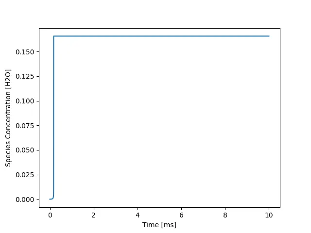
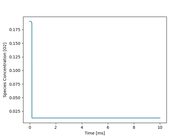
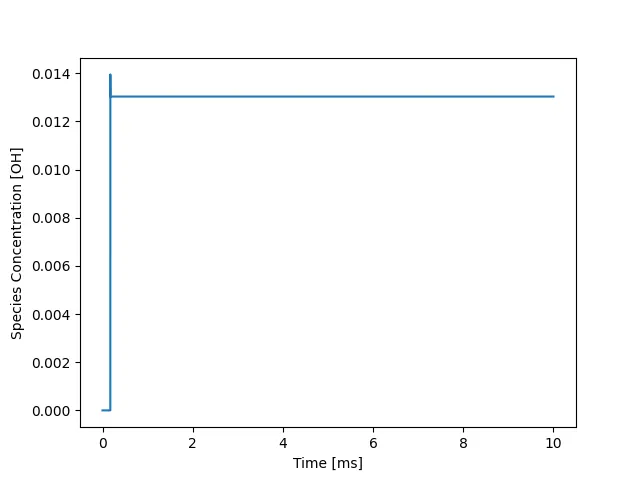
Following are the graphs for temperature of 1000K and 5bar.

CASE II:

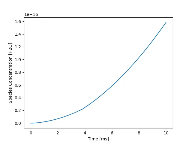
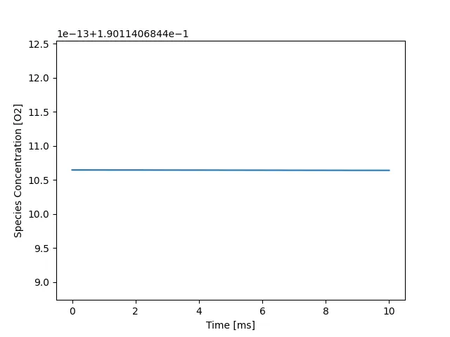
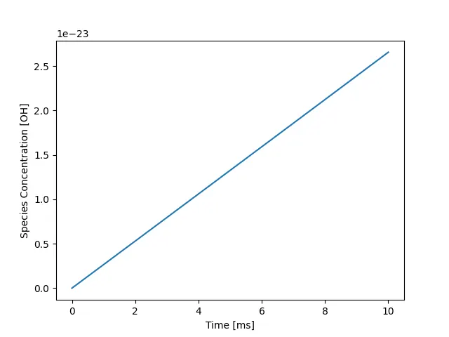
Following are the graphs for temperature of 500K and 5bar.

OBSERVATIONS:

For the temperature of 1000 K and pressure of 5 bar it can be noted that H2O concentrations were very low initially .i.e. before ignition but after ignition the concentration increased drastically showing that H2O is being formed as a product which becomes stable at the end resulting that combustion has almost reached the equilibrium stage. For the case of O2 we can see the mirrored plot of H2O which means that the reactant is being used up during the combustion. For the case of OH it can be noted that the concentration increases suddenly after some time depicting that the reaction has started and OH is formed. After sudden increase in concentration a drop can also be noted that which indicated that it is intermediate specie that is being formed during the combustion and at the same time is being consumed.

For the temperature of 500K and the pressure of 5 bar it can be noted that it can be noted that there is very little to no change in the concentration of H2O, OH, O2. This is because auto ignition temperature of methane is 873.15 and we are solving for 500K. This can also be explained as molar concentration of O2 doesn’t change which simply means that combustion hasn’t taken place. Further if we look at the plots for H2O and OH we can notice that their concentration is increasing but they don’t increase in very high order. This simply means that the auxiliary reactions are taking place but the combustion hasn’t started.