Week 7 - Auto ignition using Cantera

AIM:-

PART I

To simulate the Auto Ignition Time for Methane under the following conditions, (simulation time = 10 secs)

• Plot the variation of Auto Ignition time of Methane with a constant temperature of 1250K and pressure varying from 1 to 5 atm.
• Plot the variation of Auto Ignition time of Methane with a constant pressure of 5 atm and temperature varying from 950K to 1450K.

PART II

To observe and print the rate of change of molar concentrations of the given elements "H2O, O2, OH" with respect to the time

• When Temperature is 1000K and pressure 5 bar
• When Temperature is 500K and pressure 5 bar

Reactor Network in Cantera:-

A Cantera Reactor represents the simplest form of a chemically reacting system. It corresponds to an extensive thermodynamic control volume. in which all state variables are homogeneously distributed. The system is generally unsteady that is all the states are function of time. In particular, transient state changes due to chemical reactions are possible. However, thermodynamic equilibrium is assumed to be present throughout the reactor at all the instants of time.

Reactors can interact with the surrounding environment in multiple ways.

• Expansion/compression work:- By moving the walls of the reactor, its volume can be changed and expansion or compression work can be done by or on the reactor.
• Heat transfer:- An arbitrary heat transfer rate can be defined to cross the boundaries of the reactor.
• Mass transfer:- The reactor can have multiple inlets and outlets. For the inlets, arbitrary states can be defined. Fluid with the current state of the reactor exits the reactor at the outkets.
• Surface interaction:- One or multiple walls can influence the chemical reactions in the reactor. This is mot just restricted to catalytic reactions, but mass transfer between the surface and the fluid can also be modeled.

All of these interactions do not have to be constant, but can vary as a function of time or state.

In addition to a single reactiors. Cantera is also able to environment reactors into a reactor network. Each reactor in a network may be connected so that the contents of the reactor flow into another . Reactor may also be in contact with one another or the environment via walls that conduct heat or move to do work.

CODE:-

Part 1:-

Varying the pressure with constant temperature

import math
import matplotlib.pyplot as plt
import numpy as np
import sys
import cantera as ct

gas =ct.Solution('gri30.xml')
pressure = np.linspace(1,5,9)
T_int = 1250
time_start = 0.0
time_end =10.0
dt=1e-3
n=int((time_end-time_start)/dt)
t_autoI_P=[]
states1=[]

for i in pressure:
	gas.TPX = T_int, i*101325,{'CH4':1,'O2':2,'N2':7.52}
	T_autoI=0 
	t_autoI=0
	time=0
	r=ct.IdealGasReactor(gas)
	sim=ct.ReactorNet([r])
	states= ct.SolutionArray(gas,extra=['time_in_ms','t'])
	print('{:10s}{:10s}{:10s}'.format('t [s]','T[K]','P[Pa]'))

	for n in range(n):
		time +=1e-3
		sim.advance(time)
		states.append(r.thermo.state,time_in_ms=time*1e3,t=time)
		print('{:10.3e}{:10.3f}{:10.3f}'.format(sim.time,r.T,r.thermo.P))

	states1.append(states.T)

	for i in range(n):
		T_error = states.T[i]-T_int-400
		if T_error>0:
			T_autoI = states.T[i]
			t_autoI = states.time_in_ms[i]
			break
	t_autoI_P.append(t_autoI)

states1= np.array(states1)
for k in range (len(pressure)):
	plt.figure(1)
	plt.plot(states1[k])
	plt.xlabel('Number of timesteps')
	plt.ylabel('Temperature')
	plt.title('Variation of Auto-ignition Temperature with inlet Pressure')
	plt.legend(['1 Bar','1.5 Bar','2 Bar','2.5 Bar','3 Bar','3.5 Bar','4 Bar','4.5 Bar','5 Bar'])

plt.figure(2)
plt.plot(pressure,t_autoI_P,'b-*')
plt.xlabel('Prressure [bar]')
plt.ylabel('Auto-ignition Time [ms]')
plt.title('Ignition time delay Vs Pressure')
plt.show()

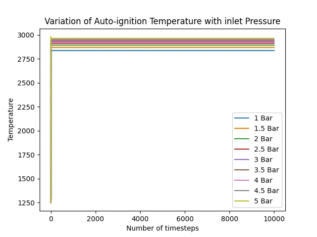
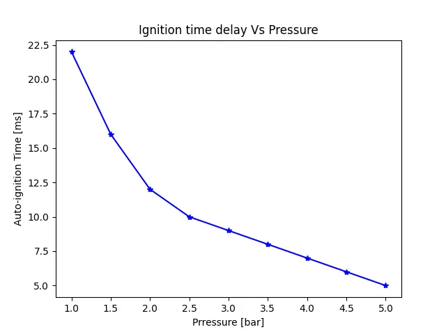
We have used gas libraries. The constant temperature used is 1250K. Took the simulation for 10 s.

We have used linspace command to variate the pressure from 1 to 5 bar.

Code for Auto ignition by varying temperature:-

import math
import matplotlib.pyplot as plt
import numpy as np
import sys
import cantera as ct

gas =ct.Solution('gri30.xml')
Temperature = np.linspace(950,1450,11)
time_start = 0.0
time_end =10.0
dt=1e-3
n=int((time_end-time_start)/dt)
t_autoI_T=[]
states1=[]

for i in Temperature:
	gas.TPX =i,5*101325,{'CH4':1,'O2':2,'N2':7.52}
	T_autoI=0 
	t_autoI=0
	time=0
	r=ct.IdealGasReactor(gas)
	sim=ct.ReactorNet([r])
	states= ct.SolutionArray(gas,extra=['time_in_ms','t'])
	print('{:10s}{:10s}{:10s}'.format('t [s]','T[K]','P[Pa]'))

	for j in range(n):
		time +=1e-3
		sim.advance(time)
		states.append(r.thermo.state,time_in_ms=time*1e3,t=time)
		print('{:10.3e}{:10.3f}{:10.3f}'.format(sim.time,r.T,r.thermo.P))

	states1.append(states.T)

	for j in range(n):
		T_error = states.T[j]-i-400
		if T_error>0:
			T_autoI = states.T[j]
			t_autoI = states.time_in_ms[j]
			break
	t_autoI_T.append(t_autoI)

states1= np.array(states1)
for k in range (len(Temperature)):
	plt.figure(1)
	plt.plot(states1[k])
	plt.xlabel('Number of timesteps')
	plt.ylabel('Temperature')
	plt.title('Variation of Auto-ignition Temperature with inlet Temperature')
	plt.legend(['950 K','1000','1050','1100','1150','1200','1250','1300','1350','1400','1450','1500'])

plt.figure(2)
plt.plot(Temperature,t_autoI_T,'r-*')
plt.xlabel('Temperature [K]')
plt.ylabel('Auto-ignition Time [ms]')
plt.title('Ignition time delay Vs Temperature')
plt.show()

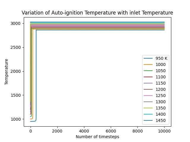
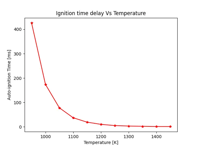
In the above code the temperature is varied from 950K to 1450 K using linspace command with constant pressure of 1.01325 bar

Case 2:-

Code for Auto ignotion by varying molar concentration

import math
import matplotlib.pyplot as plt
import numpy as np
import sys
import cantera as ct

gas =ct.Solution('gri30.xml')
T_initial = 1000
pressure= 5
n=10000
malor_conc = []

gas.TPX = T_initial,pressure*101325,{'CH4':1,'O2':2,'N2':7.52}
autoig_temp=0
autoig_time=0
r=ct.IdealGasReactor(gas)
sim= ct.ReactorNet([r])
time=0.0
states = ct.SolutionArray(gas,extra = ['time_in_ms','t'])

for n in range(n):
	time+=1e-3
	sim.advance(time)
	states.append(r.thermo.state, time_in_ms=time*1e3, t=time)

plt.subplot(3,1,1)
plt.title('Molar concentration vs Time')
plt.plot(states.t,states.X[:,gas.species_index('H2O')],'r')
plt.xlabel('time(s)')
plt.ylabel('H2O')

plt.subplot(3,1,2)
plt.plot(states.t,states.X[:,gas.species_index('O2')],'b')
plt.xlabel('time(s)')
plt.ylabel('O2')

plt.subplot(3,1,3)
plt.plot(states.t,states.X[:,gas.species_index('OH')],'g')
plt.xlabel('time(s)')
plt.ylabel('OH')

plt.show()

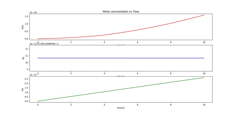
For 500K at pressure at 5 bar

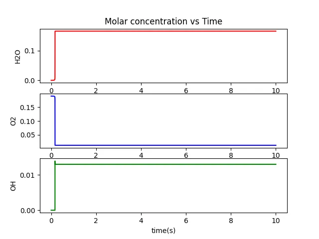
For 1000K at pressure at 5bar

CONCLUSION:-

• By varying pressure the ignition delay is getting low.
• By increasing pressure the temperature is also getting increased.
• By increasing the temperature the ignition delay is coming down.
• As you can see that the there is no change while the temoerature is at 500K but when the temperature is 1000K we see the change in molar concentration.
• So we can say that the combustion is not started at 500K instead it is getting started after increasing the temperature is greater than 500K.