Week 7 - Auto ignition using Cantera

Introduction:

Ignition delay is the time interval during which it takes from ignition temperature to 400K above it.

`Time_{"ignition delay"} = Time_{"initial temperature + 400K"}`

In the present work variation of ignition delay with pressure and temperature has been studied.

Objectives :

- Study the variation of Auto Ignition time of Methane with a constant temperature of 1250K and pressure varying from 1 to 5 atm.
- Study the variation of Auto Ignition time of Methane with a constant pressure of 5 atm and temperature varying from 950K to 1450K.

- Study of trend of change of molar concentration of H20, O2, an d OH with time at temperature of 500K and pressure 5bar, and 1000K temperature with 5 bar pressure.

Outline:

Part 1

The combustion reaction is divided into 2 sets of reaction,

A. Constant Temperature Reaction

The pressure in this case is varied from 1atm to 5 atm with a difference of 1atm at 1250K. Later the igintion temperature and ignition delay has been investigated.

B. Constant Pressure Reaction

The temperature in this case is varied from 950K to 1450K with a difference of 100K at 5atm. Later the igintion temperature and ignition delay has been investigated

Part 2

In order to investigate the products of combustion at different temperature, the study has been divided into two cases. In the first case we employ the combustion reaction at 1000K and in the second case we employ the chemical reaction at 500K.

Simulation:

The stoichiometric equation of the combustion of methan can be summarized as below:

`CH_4 + 2O_2 + 7.56N_2 = "Combustion products" dominated by CO_2 H_2O and OH`

Part 1

The following code has been developed in order to achieve the objective of Part 1

import numpy as np
import matplotlib.pyplot as plt
import cantera as ct

# Defined fucntion for calculating Ignition delays
def ign_delay(flag, T, P, t_sim):
    # variable initialized for storing ignition delay
    t_id = 0
    # defined gas as a solution class
    gas = ct.Solution('gri30.xml')
    # Initialization of Temperature Pressure and concentration
    gas.TPX = T, P, {'CH4': 1, 'O2': 2, 'N2': 7.52}
    # FLag seperating Constant pressure and constant temperature reactions for creation of reactor chamber
    if flag == "CT":
        r = ct.IdealGasReactor(gas)
    else:
        r = ct.IdealGasConstPressureReactor(gas)
    # Creating reactor network
    sim = ct.ReactorNet([r])
    
    time = 0.0
    # Marking temeprature to identify ignition
    T_combust_start = T + 400
    # Initialization of Solution array
    # Time in ms is a new variable introduced to look closely in the begining of ignition
    states = ct.SolutionArray(gas, extra = ['time_in_ms', 't'])
    for n in range(t_sim):
        time += 1e-3
        sim.advance(time)
        states.append(r.thermo.state, time_in_ms = time*1e3, t = time)
        # Conditional Statement for identifying temeperature beyond marked ignition
        if (states.T[n] <= T_combust_start):
            t_id = states.time_in_ms[n]

    return t_id, states


print("\n Constant Temperature reaction \n")

# Constant Temperature in K
temp = 1250 

# Varition of pressure in Pascal
p_start = 1 * 101325
p_end = 5 * 101325
# Difference in pressure
dP =  101325
iter = 1

t_sim = 10000
time_delay_ct = []
states_ct = []

p_i = np.arange(p_start, p_end + dP, dP)
p_atm = 101325

for i in range(len(p_i)):
    p = p_i[i]
    ignition_delay, states_temp = ign_delay("CT",temp, p, t_sim)
    time_delay_ct.append(ignition_delay)
    states_ct.append(states_temp)
 

    log_message = 'iteration = {0}, Initial Pressure = {1} atm, Initial Temperature = {2} K, Ignition Delay = {3} ms'.format(iter, p/p_atm, temp, round(ignition_delay, 2))
    print(log_message)
    iter = iter + 1



print("\n Constant Pressure reaction \n")

p = 5 * 101325 # atm

t_start = 950 # K
t_end = 1450
dt = 100
iter = 1

t_sim = 10000 # ms
time_delay_cp = []
states_cp = []

t_i = np.arange(t_start, t_end+dt, dt)

for i in range(len(t_i)):
    t = t_i[i]
    ignition_delay, states_temp = ign_delay("CP",t, p, t_sim)
    time_delay_cp.append(ignition_delay)
    states_cp.append(states_temp)

    log_message = 'iteration = {0}, Initial Pressure = {1} atm, Initial Temperature = {2} K, Ignition Delay = {3} ms'.format(iter, p/p_atm, t, round(ignition_delay, 2))
    print(log_message)
    iter = iter + 1


# Plotting data for Constant Temperature Ignition Delays

plt.figure(1)
t = [i.t for i in states_ct]
T = [i.T for i in states_ct]
for i in range(5):
    plt.plot(t[i], T[i])
plt.title("1. Variation of Temperature with Time")
plt.xlabel("Time (s)")
plt.ylabel("Temperature (K)")
plt.legend(['Initial Pressure = ' + str(p) + ' atm' for P in p_i/101325])
plt.show(block = False)

plt.figure(2)
time_in_ms = [i.time_in_ms for i in states_ct]
for i in range(5):
    plt.plot(time_in_ms[i], T[i])
plt.xlim(0, 30)
plt.title("2. Variation of Temperature with Time")
plt.xlabel("Time [ms]")
plt.ylabel("Temperature [K]")
plt.legend(['Initial Pressure = ' + str(p) + ' atm' for P in p_i/101325])
plt.show(block=False)

plt.figure(3)
plt.plot(p_i/101325, time_delay_ct, marker = 'o')
plt.title("3. Effect of Variation in Initial Pressure on Ignition Delay")
plt.xlabel("Pressure [atm]")
plt.ylabel("Ignition Delay [ms]")
plt.show(block = False)


# Plotting data for Constant Pressure Ignition Delays

plt.figure(4)
t = [i.t for i in states_cp]
T = [i.T for i in states_cp]
for i in range(6):
    plt.plot(t[i], T[i])
plt.title("4. Variation of Temperature with Time")
plt.xlabel("Time [s]")
plt.ylabel("Temperature [K]")
plt.legend(['Initial Temperature = ' + str(T) + ' K' for T in t_i])
plt.show(block = False)

plt.figure(5)
time_in_ms = [i.time_in_ms for i in states_cp]
for i in range(6):
    plt.plot(time_in_ms[i], T[i])
plt.xlim(0, 500)
plt.title("5. Variation of Temperature with Time")
plt.xlabel("Time [ms]")
plt.ylabel("Temperature [K]")
plt.legend(['Initial Temperature = ' + str(T) + ' K' for T in t_i])
plt.show(block = False)

plt.figure(6)
plt.plot(t_i, time_delay_cp, marker = 'o')
plt.title("6. Effect of Variation in Initial Temperature on Ignition Delay")
plt.xlabel("Temperature [K]")
plt.ylabel("Ignition Delay [ms]")
plt.show()

Constant Temperature Reaction

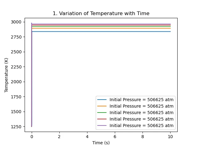
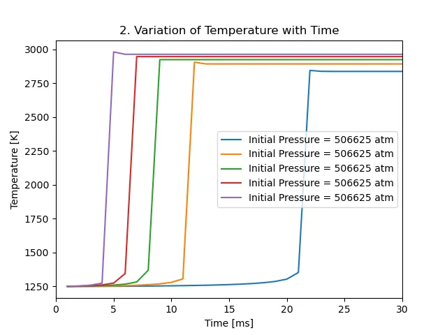
For a closer look at the ignition process in the begining of reaction, temperature vs time is plotted for 30 ms.

Constant Pressure Reaction

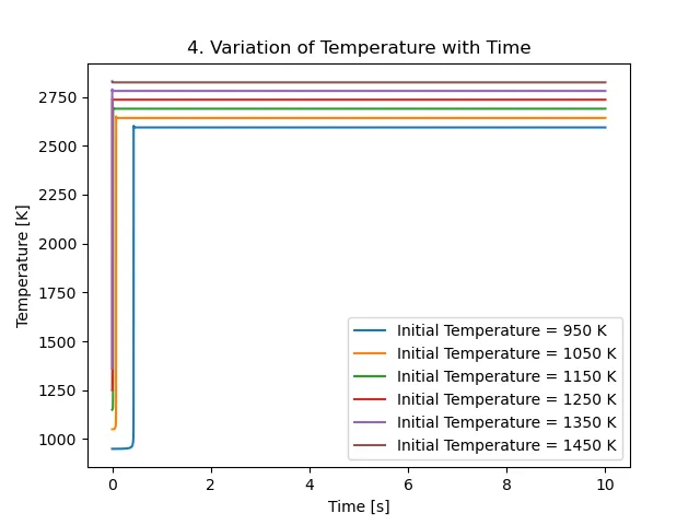
For a closer look at the ignition process in the begining of reaction, temperature vs time is plotted for 500 ms.

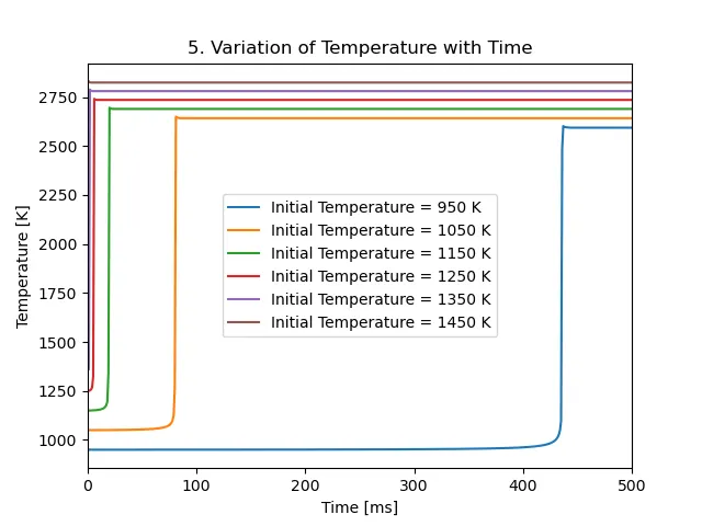
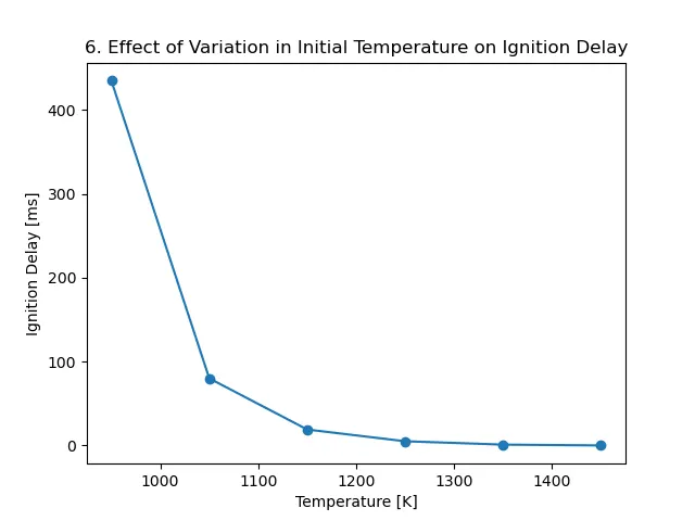
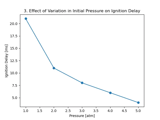
At constant pressure reaction, after observing the plot, it is evident that, increase in initial temperature reduces the ignition delay and increases maximum temperature. Simular behaviour can be observed in the constant temperature reaction.
In the case of constant pressure reaction, the reduction in ignition delay is much faster as compared to constant temperature combustion.

Part 2

The foloowing code has been developed in the study of part 2

import sys
import numpy as np
import matplotlib.pyplot as plt
import cantera as ct

# Given constant pressure
p = 5 * 1e5 
# Defined Temeprature array 
T = [1000, 500] # K

# Simulation time iteration
t_sim = 10000 # ms

# Defined function for species concentration
def species_conc(T):
    gas = ct.Solution('gri30.xml')
    gas.TPX = T,p,{'CH4': 1, 'O2': 2, 'N2': 7.52}
    r = ct.IdealGasReactor(gas)
    
    sim = ct.ReactorNet([r])
    time = 0.0
    
    states = ct.SolutionArray(gas, extra = ['time_in_ms', 't'])
    for n in range(t_sim):
        time += 1e-3
        sim.advance(time)
        states.append(r.thermo.state, time_in_ms = time*1e3, t = time)
# Saving the values of concentration of species 
    species_H2O = states.X[:, gas.species_index('H2O')]
    species_O2 = states.X[:, gas.species_index('O2')]
    species_OH = states.X[:, gas.species_index('OH')]
    
    return species_H2O, species_O2, species_OH, states


for i,j in enumerate(T):
    species_H2O, species_O2, species_OH, states = species_conc(j)
    plt.figure(i+1)
    plt.plot(states.t, species_H2O, color = 'b')
    plt.plot(states.t, species_O2, color = 'r')
    plt.plot(states.t, species_OH, color = 'y')
    plt.title("Effect of Variation of Mole Fractions of Species \n at different instances of time at temperature {0} K".format(str(j)))
    plt.xlabel("Time [s]")
    plt.ylabel("Mole Fractions of Species")
    plt.legend(["H2O", "O2", "OH"])
    plt.show(block=False)
    

plt.show()

In the combustion process there are many products that are released, including pollutants. Among them CO2, H2O and OH are most predominant.

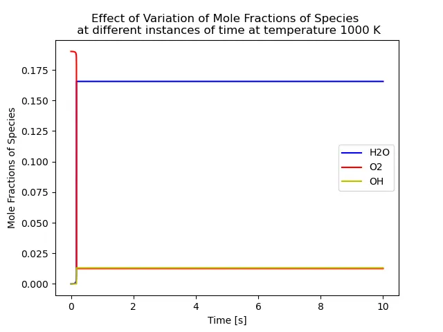
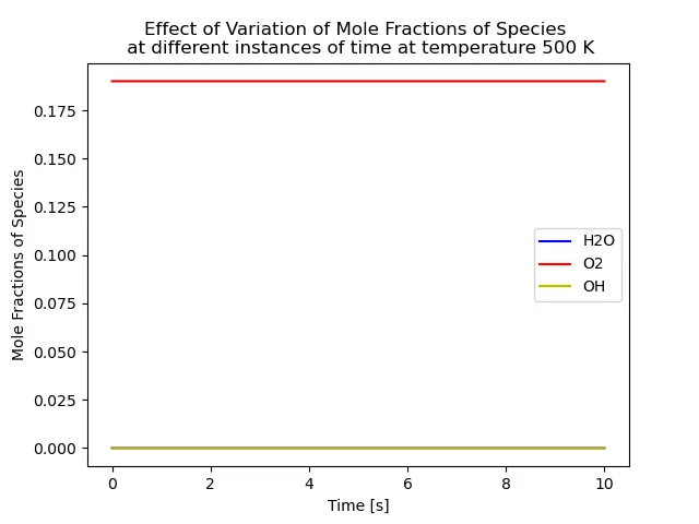
From the plot it can be seen that mole fraction of species remain same until end of the time for temperature of 500K. The phenomenon can be attributed to the temperature lower than the ignition temperature.

When the combustion starts, the concentration of O2 decreases at a rapid rate and the products symbolized by formation of H2O can be seen along with OH. This marks a sucessful combustion unlike in the case of temperated at 500K