Week 7 - Auto ignition using Cantera
Auto Ignition using Cantera
- Aim :
- Calculate auto ignition delay for methane using Cantera.
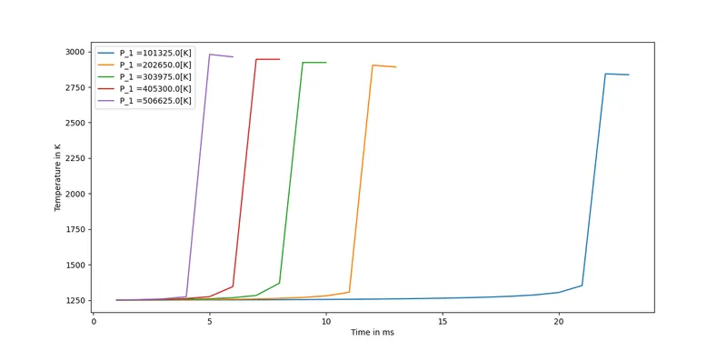
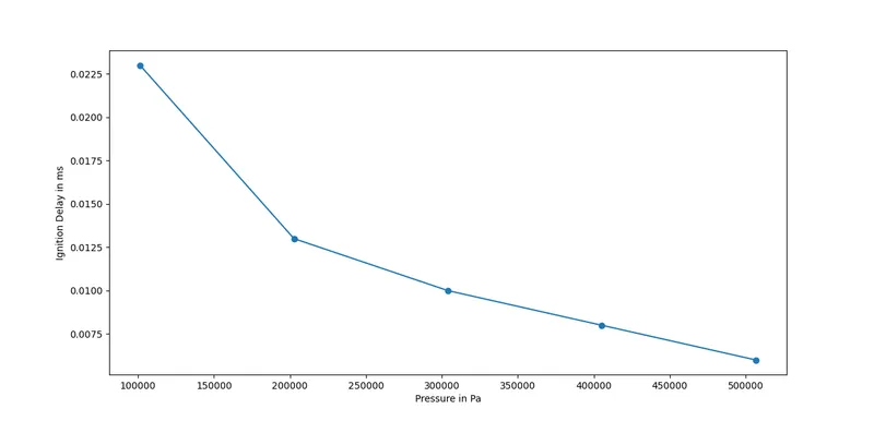
- Plot the variation of Auto Ignition time of Methane with a constant temperature of 1250K and pressure varying from 1 to 5 atm.
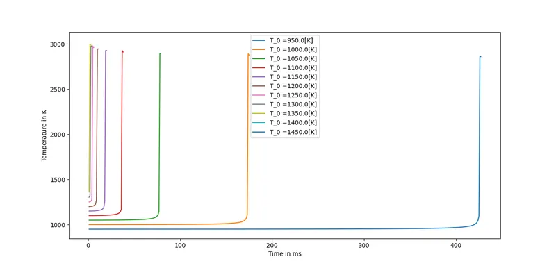
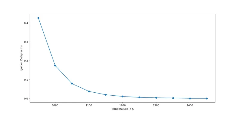
- Plot the variation of Auto Ignition time of Methane with a constant pressure of 5 atm and temperature varying from 950K to 1450K.
- Observe and print the rate of change of molar concentrations of the given elements "H2O, O2, OH" with respect to the time when Temperature is 1000K and pressure 5 bar.
- Observe and print the rate of change of molar concentrations of the given elements "H2O, O2, OH" with respect to the time when Temperature is 500K and pressure 5 bar.
- Theory :
Auto Ignition - The autoignition temperature or kindling point of a substance is the lowest temperature in which it spontaneously ignites in a normal atmosphere without an external source of ignition, such as a flame or spark. This temperature is required to supply the activation energy needed for combustion. The temperature at which a chemical ignites decreases as the pressure or oxygen concentration increases. It is usually applied to a combustible fuel mixture.
Auto Ignition Delay - The autoignition delay time, τ ( T , p ) , is the time for which a homogeneous mixture must be maintained at temperature, T, and pressure, p, before it autoignites. The longer ignition delay can be caused by a number of factors including: lower intake air temperature, lower boost pressure due to turbocharger lag, lower combustion chamber wall temperature and more advanced dynamic injection timing.
- Steps involved in coding :
- Import numpy, matplotlib, sys and cantera module.
- Create gas object in solution class.
- Define values of temperature and pressure for different cases.
- Create a 'for' loop for values of temperature or pressure.
- Use 'gas.TPX' command and define values of temperature, pressure and mole fractions of species.
- Create a reactor object named 'r' using 'ct.IdealGasReactor' command.
- Define starting time and end time of simulation. In this case the simulation is ran for 10 seconds.
- Create 'states' object to store different properties. It is used as solution array.
- Create time loop and integrate the solution after 1e-3 seconds.
- Create 'if' loop to calculate ignition delay.
- Plot the results for different cases.
- Part I :
Case A -
import sys
import numpy as np
import matplotlib.pyplot as plt
import cantera as ct

gas = ct.Solution('gri30.xml')

T = 1250
P_1 = 1*101325
P_5 = 5*101325
Pressure = np.linspace(P_1,P_5,5)
Ignition_delay = []
for P in Pressure:

	gas.TPX = T, P, {'CH4':1, 'O2':2, 'N2':7.52}

	r = ct.IdealGasReactor(gas)
	sim = ct.ReactorNet([r])
	time = 0.0
	T_old = T
	states = ct.SolutionArray(gas, extra=['time_in_ms', 't'])
	states_temperature = []
	#Ignition_delay = []
	for n in range(10000):
		time += 1e-3
		sim.advance(time)
		states.append(r.thermo.state, time_in_ms = time*1e3, t = time)
		T_new = states.T
		T_new = T_new[n-1]

		if T_new>= T_old + 400:
			Ignition_delay.append(time)
			T_old = states.T
			T_old = T_old[n-1]

			plt.figure(1)
			plt.plot(states.time_in_ms, states.T)


print('Ignition Delay=', Ignition_delay)
print('Pressure=', Pressure)


plt.xlabel('Time in ms')
plt.ylabel('Temperature in K')
plt.legend(['P_1 =' + str(P) + '[K]' for P in Pressure])


plt.figure(2)
plt.plot(Pressure, Ignition_delay, '-o')
plt.xlabel('Pressure in Pa')
plt.ylabel('Ignition Delay in ms')
plt.show()
Plots -
Plot of temperature vs time when pressure is varied.
Plot of ignition delay when pressure is varied.
Results -
Ignition Delay= [0.023000000000000013, 0.013000000000000005, 0.010000000000000002, 0.008, 0.006]
Pressure= [101325. 202650. 303975. 405300. 506625.]
From the above plotswe can see that the Ignition delay time reduces as we increase the pressure. Lowest ignition delay time is noted at pressure of 5 bar. This means that ignition delay is dependant on pressure.
Case B -
import sys
import numpy as np
import matplotlib.pyplot as plt
import cantera as ct

gas = ct.Solution('gri30.xml')

T_0 = 950
T_n = 1450
P = 5*101325
Temperature = np.linspace(T_0,T_n,11)
Ignition_delay = []
for T in Temperature:

	gas.TPX = T, P, {'CH4':1, 'O2':2, 'N2':7.52}

	r = ct.IdealGasReactor(gas)
	sim = ct.ReactorNet([r])
	time = 0.0
	T_old = T
	states = ct.SolutionArray(gas, extra=['time_in_ms', 't'])
	states_temperature = []
	#Ignition_delay = []
	for n in range(10000):
		time += 1e-3
		sim.advance(time)
		states.append(r.thermo.state, time_in_ms = time*1e3, t = time)
		T_new = states.T
		T_new = T_new[n-1]

		if T_new>= T_old + 400:
			Ignition_delay.append(time)
			T_old = states.T
			T_old = T_old[n-1]

			plt.figure(1)
			plt.plot(states.time_in_ms, states.T)


print('Ignition Delay=', Ignition_delay)
print('Temperature=', Temperature)


plt.xlabel('Time in ms')
plt.ylabel('Temperature in K')
plt.legend(['T_0 =' + str(T) + '[K]' for T in Temperature])


plt.figure(2)
plt.plot(Temperature, Ignition_delay, '-o')
plt.xlabel('Temperature in K')
plt.ylabel('Ignition Delay in ms')
plt.show()
Plots -
Plot of temperature vs time when temperature is varied.
Plot of Ignition delay vs Temperature.
Results -
Ignition Delay= [0.4270000000000003, 0.17500000000000013, 0.07900000000000006, 0.03800000000000003, 0.02000000000000001, 0.011000000000000003, 0.006, 0.004, 0.003, 0.001, 0.001]
Temperature= [ 950. 1000. 1050. 1100. 1150. 1200. 1250. 1300. 1350. 1400. 1450.]
From the above plots and results it is observed that ignition delay time reduces when fuel temperature is high. This means the ignition delay time is dependant on temperature. When temperature is at 1450 K the ignition delay is lowest.
- Part II :
Case A -
import sys
import numpy as np
import matplotlib.pyplot as plt
import cantera as ct

gas = ct.Solution('gri30.xml')

T = 1000
P = 5*101325

Ignition_delay = []


gas.TPX = T, P, {'CH4':1, 'O2':2, 'N2':7.52}

r = ct.IdealGasReactor(gas)
sim = ct.ReactorNet([r])
time = 0.0
T_old = T
states = ct.SolutionArray(gas, extra=['time_in_ms', 't'])
states_temperature = []
#Ignition_delay = []
for n in range(10000):
	time += 1e-3
	sim.advance(time)
	states.append(r.thermo.state, time_in_ms = time*1e3, t = time)


plt.figure(1)
plt.plot(states.time_in_ms, states.X[:, gas.species_index("H2O")])
plt.xlabel("Time in ms")
plt.ylabel("Species concentration of H2O")

plt.figure(2)
plt.plot(states.time_in_ms, states.X[:, gas.species_index("O2")])
plt.xlabel("Time in ms")
plt.ylabel("Species concentration of O2")

plt.figure(3)
plt.plot(states.time_in_ms, states.X[:, gas.species_index("OH")])
plt.xlabel("Time in ms")
plt.ylabel("Species concentration of OH")
plt.show()
Plots -
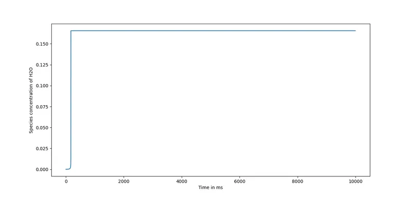
Plot of concentration of H2O vs simulation time.
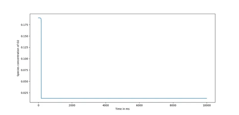
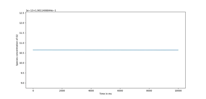
Plot of concentration of O2 vs simulation time.
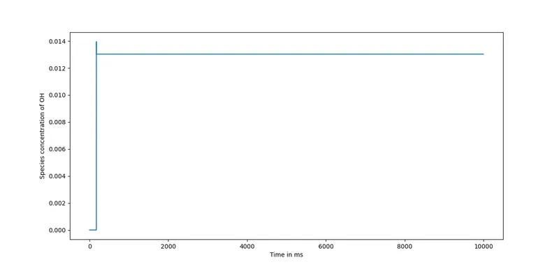
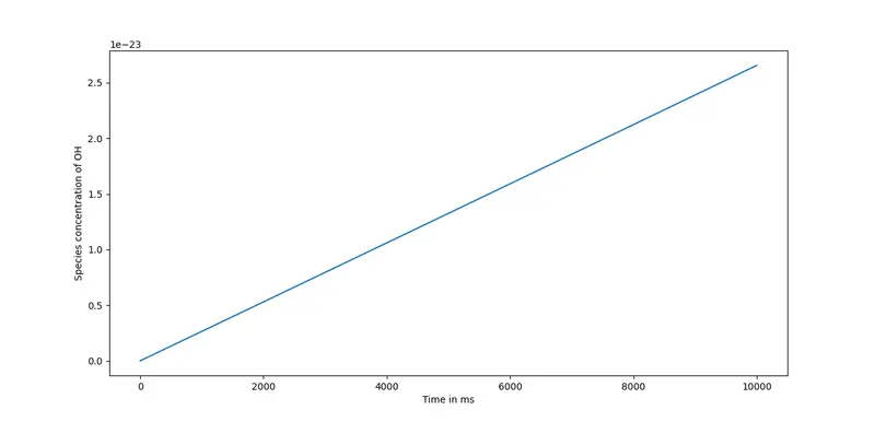
Plot of concentration of OH vs simulation time.
Results -
- Initially concentration is low. Then concentration of H2O increases suddenly after few mili-seconds and then remains same for rest for the simulation time.
- Concentration of O2 is high at the begining. Then it suddenly decreases and remains constant for rest of the simulation time.
- Concentration of OH is low at the start. Then a sudden spike is observed but soon it reduces a little and then remains steady for rest of the simulation.
Case B -
import sys
import numpy as np
import matplotlib.pyplot as plt
import cantera as ct

gas = ct.Solution('gri30.xml')

T = 500
P = 5*101325

Ignition_delay = []


gas.TPX = T, P, {'CH4':1, 'O2':2, 'N2':7.52}

r = ct.IdealGasReactor(gas)
sim = ct.ReactorNet([r])
time = 0.0
T_old = T
states = ct.SolutionArray(gas, extra=['time_in_ms', 't'])
states_temperature = []
#Ignition_delay = []
for n in range(10000):
	time += 1e-3
	sim.advance(time)
	states.append(r.thermo.state, time_in_ms = time*1e3, t = time)


plt.figure(1)
plt.plot(states.time_in_ms, states.X[:, gas.species_index("H2O")])
plt.xlabel("Time in ms")
plt.ylabel("Species concentration of H2O")

plt.figure(2)
plt.plot(states.time_in_ms, states.X[:, gas.species_index("O2")])
plt.xlabel("Time in ms")
plt.ylabel("Species concentration of O2")

plt.figure(3)
plt.plot(states.time_in_ms, states.X[:, gas.species_index("OH")])
plt.xlabel("Time in ms")
plt.ylabel("Species concentration of OH")
plt.show()
Plots -
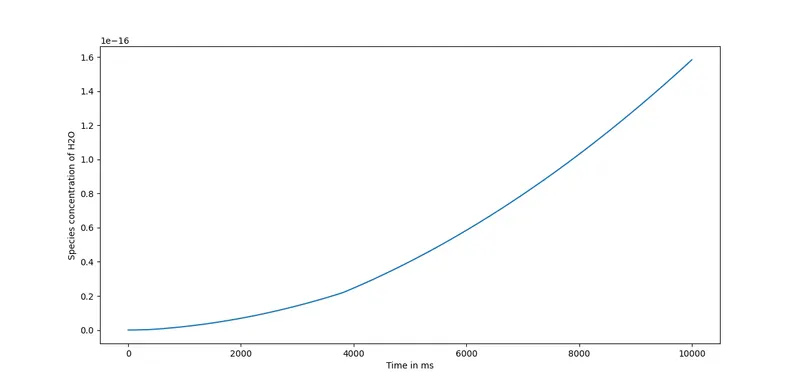
Results -
- Concentration of H2O is intially low but it steadily increases as the simulation time keeps on increasing.
- Concentration of O2 remains constant throughout the simulation.
- Concentration fo OH increases linearly as the simulation time keeps on increasing.
- Conclusion :
- Auto ignition is dependant on pressure and change in pressure can be utilized toadjust auto ignition delay.
- Temperature of fuel affects the auto igition. If temperature is high, the fuel ignites quickly.
- The concentration of species varies when temperature of methane is varied.