Week 7 - Auto ignition using Cantera
study Methane (CH4) of Ignition delay at the various condition for 10 seconds
Given Data
Part 1
Case 1a
constant temperature T=1250 k
variable pressure varies from P= 1 to 5 bar
case 1b
constant pressure P=5 bar
variable Temperature varies from T=950 to 1450k
Part 2
case2a
constant Temperature T=500k
constant Pressure P=5 bar
case2b
constant Temperature T=1000k
constant Pressure P=5 bar
To Find
ignition delay time for 10 seconds
case 1
Auto Ignition time of Methane for a given condition with respect to time
case 2
molar concentrations H2O, O2, OH of given condition with respect to time
Solution
by using Cantera inbuilt combustion Data analysis are carried out at different condition by just adding input function data to Cantera to analyse the objective to solve the problem
Autoignition temperature
- is the temperature at which a material spontaneously ignites in a normal atmosphere without an external source of ignition.
- is the temperature required to supply the activation energy for combustion
- is usually applied to combustible fuel mixtures
- The ignition temperature of a substance is the least temperature at which the substance starts combustion
Auto Ignition time is the time when the temperature of the reactor is Initial Temperature plus 400K
`T_(AUTOIGNITION)=T_(INITIAL)+400K`
solving using Cantera & Python for the given condition
Python cantera code
"""
Ignition Delay analysis for various condition
 Auto Ignition Time for Methane under the following conditions for 10 secounds analysis

 Case1
case1 a
 Plot the variation of Auto Ignition time of Methane with a constant temperature of 1250K and pressure varying from 1 to 5 atm.
case1 b
 Plot the variation of Auto Ignition time of Methane with a constant pressure of 5 atm and temperature varying from 950K to 1450K.

Case2
molar concentrations of the given elements "H2O, O2, OH" with respect to the time
case2 a
When Temperature is 1000K and pressure 5 bar
case2 b
When Temperature is 500K and pressure 5 bar


Program by S.Jagaveerapandiyan
"""
import sys
import numpy as py
import cantera as ct
import numpy as np
import matplotlib.pyplot as plt

gas=ct.Solution('gri30.xml')
T=np.linspace(950,1450,51)
P=101325*(np.linspace(1,5,9))
t=np.linspace(0,10,10001)
species={'CH4':1,'O2':2,'N2':7.52}
Tm=[500,1000]
T_C=[]
def auto_ignition(T,P,spicies,t):
	gas.TPX=T,P,species
	r=ct.IdealGasReactor(gas)
	sim=ct.ReactorNet([r])
	states=ct.SolutionArray(gas,extra=['time_in_ms','t'])

	# creating Time loop
	for n in t:
		sim.advance(n)
		states.append(r.thermo.state, time_in_ms=n*1e3,t=n*1e-3)
	return states

#output
#time
#case 1a
T_in_T=[[0 for time in t] for temp in T]

#case 1b
P_in_T=[[0 for time in t] for press in P]

#case 2a,b
C_T=[[0 for time in t] for i in range(0,2)]

# storing variable with function of time
time_fun_T=[]
time_fun_P=[]

# case 2 molar concentration
molefraction1=[[0 for time in t] for i in range(0,3)]
molefraction2=[[0 for time in t] for i in range(0,3)]

# Solution
# case 1a
print('Variable Pressure at maximum Autoignition Temperature')
for i in range(0,len(P)):
	states=auto_ignition(T[30],P[i],species,t)
	P_in_T[i]=states.T
	print(P[i]/101325,'bar''=',np.max(P_in_T),'k')
	# constraining auto ignition condition
	for n in range(0,len(states.T)):
		if states.T[n]>=states.T[0]+400:
			time_fun_P.append(states.time_in_ms[n])
			break

# plotting case 1a1
fig1,ax1=plt.subplots()

for i in range(0,len(P)):
	plt.plot(t,P_in_T[i],label=str(P[i]/101325)+'atm')


plt.xlabel('time [sec]',fontsize=13)
plt.ylabel('Temperature [K]',fontsize=13)
plt.title('Reaction Temperature with variable Pressure',fontsize=16,fontweight='bold')
plt.grid('both',linestyle='--',linewidth=0.5)
plt.legend(fontsize=13)
plt.savefig('case1_CT1.png')

# plotting case 1a2
fig2,ax2=plt.subplots()

plt.plot(P/101325,time_fun_P,'r','-*')
plt.xlabel('Pressure [atm]',fontsize=13)
plt.ylabel('Ignition delay [ms]',fontsize=13)
plt.title('Ignition delay with variable Temperature',fontsize=16,fontweight='bold')
ax2.yaxis.set_major_locator(plt.MaxNLocator(10))
plt.yticks(rotation = 0)
plt.grid('both',linestyle='--',linewidth=0.5)
plt.legend(fontsize=13)
plt.savefig('case1_CT2.png')
# Solution
# case 1b
print('Variable initial Temperature to maximum Autoignition Temperature')
for i in range(0,len(T)):
	states=auto_ignition(T[i],P[-1],species,t)
	T_in_T[i]=states.T
	print(T[i],'k','=',np.max(T_in_T),'k')
	for n in range(0,len(states.T)):
		if states.T[n]>=states.T[0]+400:
			time_fun_T.append(states.time_in_ms[n])
			break

# plotting case 1b1
fig3,ax3=plt.subplots()
for i in range(0,len(P)):
	plt.plot(t,T_in_T[i],label=str(T[i])+'K')

plt.xlabel('time [sec]',fontsize=13)
plt.ylabel('Temperature [K]',fontsize=13)
plt.title('Reaction Temperature with variable initial Temperature',fontsize=16,fontweight='bold')
plt.grid('both',linestyle='--',linewidth=0.5)
plt.legend(fontsize=13)
plt.savefig('case1b1_CT1.png')

# plotting case 1a2
fig4,ax4=plt.subplots()

plt.plot(T,time_fun_T,'r','-*')
plt.xlabel('Temperature [k]',fontsize=13)
plt.ylabel('Ignition delay [ms]',fontsize=13)
plt.title('Ignition delay with variable Temperature',fontsize=16,fontweight='bold')
plt.grid('both',linestyle='--',linewidth=0.5)
plt.legend(fontsize=13)
plt.savefig('case1a2_ig.png')
plt.xlim([T[0],T[-1]])
ax4.yaxis.set_major_locator(plt.MaxNLocator(10))
plt.yticks(rotation = 10)
plt.savefig('case1a2_CP2.png')

print(np.max(time_fun_T))
#case 2a
states=auto_ignition(Tm[0],P[-1],species,t)
molefraction1[0]=states.X[:,states.species_index('H2O')]
molefraction1[1]=states.X[:,states.species_index('O2')]
molefraction1[2]=states.X[:,states.species_index('OH')]
C_T[0]=states.T

#plotting case2a
fig5,ax5=plt.subplots(3)
ax5[0].plot(t,molefraction1[0],'r')
ax5[1].plot(t,molefraction1[1],'r')
ax5[2].plot(t,molefraction1[2],'r')
plt.suptitle('Mole Fractions for reaction at 500 k & 5 bar')
ax5[0].set_ylabel('$X_{H_2O}$',fontsize=13)
ax5[1].set_ylabel('$X_{O_2}$',fontsize=13)
ax5[2].set_ylabel('$X_{OH}$',fontsize=13)
ax5[2].set_xlabel('Time [sec]',fontsize=13)
ax5[0].grid('both',linestyle='--',linewidth=0.5)
ax5[1].grid('both',linestyle='--',linewidth=0.5)
ax5[2].grid('both',linestyle='--',linewidth=0.5)
plt.savefig('case2a1_x.png')

# printing maximum concentration of species
print('maximum concentration of species 500k 5bar')
print('H_2O=',np.max(molefraction1[0]))
print('O_2=',np.max(molefraction1[1]))
print('OH=',np.max(molefraction1[2]))

# printing minimum concentration of species
print('maximum concentration of species 500k 5bar')
print('H_2O=',np.min(molefraction1[0]))
print('O_2=',np.max(molefraction1[1]))
print('OH=',np.max(molefraction1[2]))
#case 2b
states=auto_ignition(Tm[-1],P[-1],species,t)
molefraction2[0]=states.X[:,states.species_index('H2O')]
molefraction2[1]=states.X[:,states.species_index('O2')]
molefraction2[2]=states.X[:,states.species_index('OH')]
C_T[1]=states.T


#plotting case2b
fig6,ax6=plt.subplots(3)
ax6[0].plot(t,molefraction2[0],'r')
ax6[1].plot(t,molefraction2[1],'r')
ax6[2].plot(t,molefraction2[2],'r')
plt.suptitle('Mole Fractions for reaction at 1000 k & 5 bar')
ax6[0].set_ylabel('$X_{H_2O}$',fontsize=13)
ax6[1].set_ylabel('$X_{O_2}$',fontsize=13)
ax6[2].set_ylabel('$X_{OH}$',fontsize=13)
ax6[2].set_xlabel('Time [sec]',fontsize=13)
ax6[0].grid('both',linestyle='--',linewidth=0.5)
ax6[1].grid('both',linestyle='--',linewidth=0.5)
ax6[2].grid('both',linestyle='--',linewidth=0.5)
plt.savefig('case2b1_x.png')

# printing maximum concentration of species
print('maximum concentration of species 1000k 5bar')
print('H_2O=',np.max(molefraction2[0]))
print('O_2=',np.max(molefraction2[1]))
print('OH=',np.max(molefraction2[2]))

# printing minimum concentration of species
print('maximum concentration of species 1000k 5bar')
print('H_2O=',np.min(molefraction2[0]))
print('O_2=',np.max(molefraction2[1]))
print('OH=',np.max(molefraction2[2]))

#Auto ignition plotting
print('maximum temperature at 5 bar,1000k')
fig7,ax7=plt.subplots()
for i in range(0,2):
	plt.plot(t,C_T[i],label=str(Tm[i])+'K')
	print(np.max(C_T[i]))
plt.xlabel('Time [sec]',fontsize=13)
plt.ylabel('Temperature [K]',fontsize=13)
plt.title('Reaction Temperature with variable initial Temperature')
plt.grid('both',linestyle='--',linewidth=0.5)
plt.legend(fontsize=10)
plt.savefig('ig.png')

plt.show()
Result
case1 a
The reaction of temperature at variable Pressure time Vs Temperature
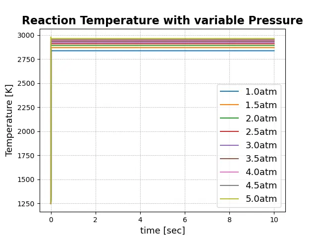
Detail View
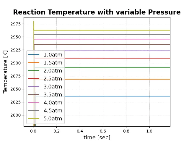
Maximum Temperature with respect to Pressure
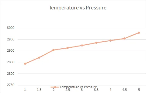
the above graph for maximum temperature with the function of initial Pressure given below
| Points | Pressure(bar) | Temperature (K) |
| 1 | 1 | 2843.425961 |
| 2 | 1.5 | 2870.43795 |
| 3 | 2 | 2903.912127 |
| 4 | 2.5 | 2912.895224 |
| 5 | 3 | 2923.149813 |
| 6 | 3.5 | 2935.044279 |
| 7 | 4 | 2945.332147 |
| 8 | 4.5 | 2954.493342 |
| 9 | 5 | 2979.948726 |
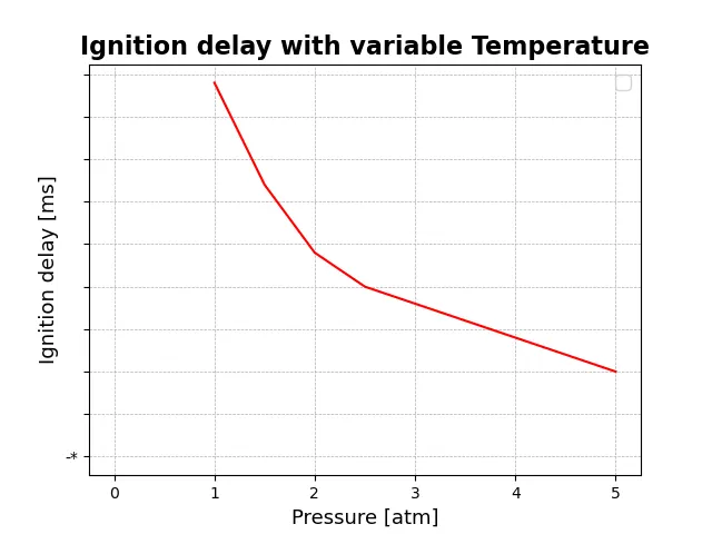
case1 a
Ignition Delay VS Pressure with various Temperature
case 1 b
Temperature Vs Time at variable Initial Temperature
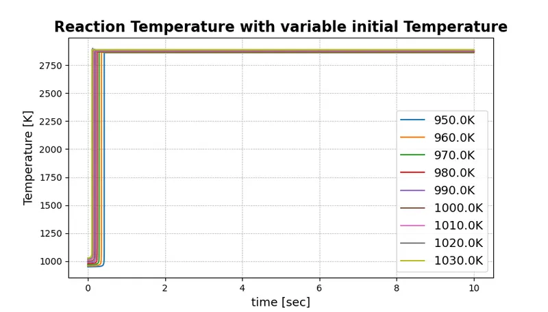
Detail view
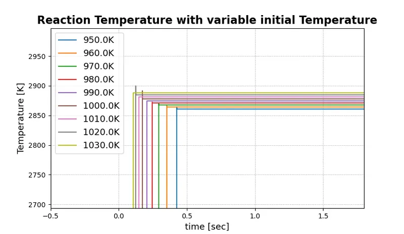
maximum Ignition Temperature with the function of Initial Temperature
the above graph for maximum temperature with the function of initial temperature given below
| Points | Initial Temperature (K) | Ignition Temperature (K) |
| 1 | 950 | 2864.395148 |
| 2 | 960 | 2867.846787 |
| 3 | 970 | 2869.870487 |
| 4 | 980 | 2872.357707 |
| 5 | 990 | 2874.53726 |
| 6 | 1000 | 2891.64114 |
| 7 | 1010 | 2891.64114 |
| 8 | 1020 | 2899.887006 |
| 9 | 1030 | 2899.887006 |
| 10 | 1040 | 2899.887006 |
| 11 | 1050 | 2899.887006 |
| 12 | 1060 | 2901.211085 |
| 13 | 1070 | 2901.8416 |
| 14 | 1080 | 2905.324338 |
| 15 | 1090 | 2910.487157 |
| 16 | 1100 | 2928.608197 |
| 17 | 1110 | 2928.608197 |
| 18 | 1120 | 2928.608197 |
| 19 | 1130 | 2928.608197 |
| 20 | 1140 | 2928.608197 |
| 21 | 1150 | 2928.608197 |
| 22 | 1160 | 2932.198126 |
| 23 | 1170 | 2955.271056 |
| 24 | 1180 | 2955.271056 |
| 25 | 1190 | 2955.271056 |
| 26 | 1200 | 2955.271056 |
| 27 | 1210 | 2955.271056 |
| 28 | 1220 | 2955.271056 |
| 29 | 1230 | 2955.271056 |
| 30 | 1240 | 2959.414182 |
| 31 | 1250 | 2959.414182 |
| 32 | 1260 | 2959.414182 |
| 33 | 1270 | 2959.414182 |
| 34 | 1280 | 2959.414182 |
| 35 | 1290 | 2959.414182 |
| 36 | 1300 | 2959.414182 |
| 37 | 1310 | 2982.305284 |
| 38 | 1320 | 2985.601769 |
| 39 | 1330 | 2997.743691 |
| 40 | 1340 | 2997.743691 |
| 41 | 1350 | 2997.743691 |
| 42 | 1360 | 2997.743691 |
| 43 | 1370 | 3002.050005 |
| 44 | 1380 | 3005.324502 |
| 45 | 1390 | 3027.888725 |
| 46 | 1400 | 3027.888725 |
| 47 | 1410 | 3027.888725 |
| 48 | 1420 | 3027.888725 |
| 49 | 1430 | 3027.888725 |
| 50 | 1440 | 3027.888725 |
| 51 | 1450 | 3027.888725 |
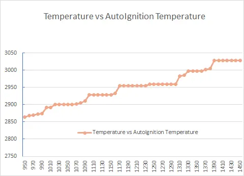
Gradual increases in ignition time with initial time shown above
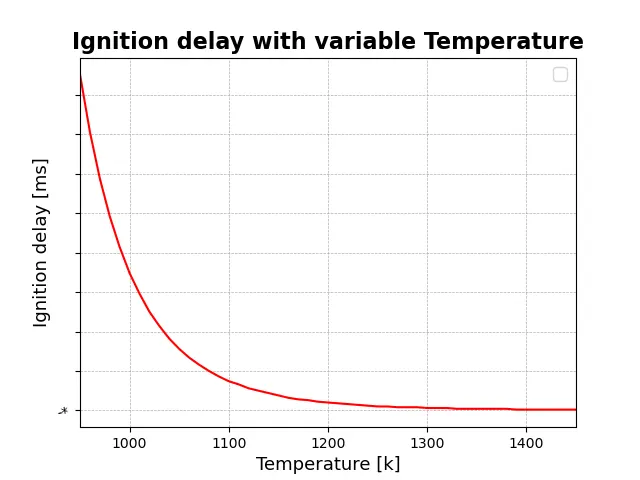
Case 1b
Temperature Vs Ignition Delay with variable initial Temperature
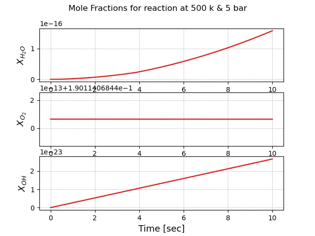
Case2 a
The molar concentration OF H2O, O2, OH varies Vs time with constant Pressure 5 Bar & Constant initial Temperature of 500K
Case2 a
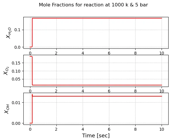
The molar concentration OF H2O, O2, OH varies Vs time with constant Pressure 5 Bar & Constant initial Temperature of 1000K
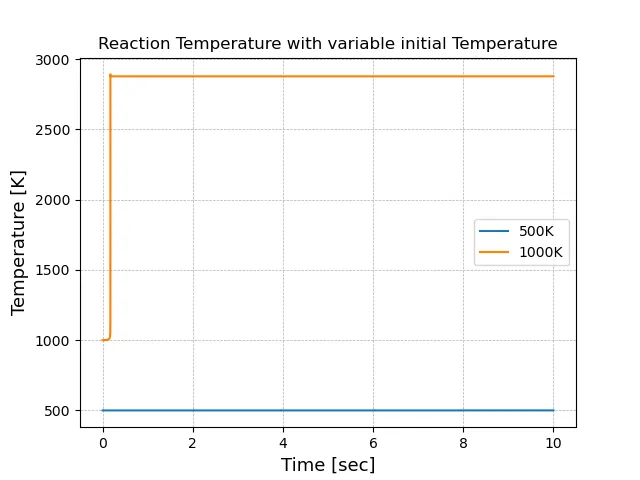
Variable Initial Temperature VS Time
case1a
Frome absorbed in the graph
At 5bar=2979.948726 k ignition temperature which is faster in time than all Pressure
so when pressure is a function of time if is increases ignition delay time decreases
`Ppropto(1/T_(IGNITION DELAY))`
case1b
Frome absorbed in the graph
At From 1380k the ignition delay is constant at lesser time which is maximum 3027.88k after that it become constant
`T_(INITIAL)propto(1/T_(IGNITION DELAY))`
case2a
molar Fraction for different species
maximum concentration of species
H_2O= 1.58442590583662e-16
O_2= 0.19011406844106465
OH= 2.655661879743359e-23
maximum concentration of species
H_2O= 0.0
O_2= 0.19011406844106465
OH= 2.655661879743359e-23
case2b
maximum concentration of species
H_2O= 0.16567020336733546
O_2= 0.19011406844106465
OH= 0.013952869738833114
maximum concentration of species
H_2O= 0.0
O_2= 0.19011406844106465
OH= 0.013952869738833114
from the absoube from graph Maximum Ignition Temperature for 1000K 5bar is 2891.641 k
Source
Skill lync Team