Week 7 - Auto ignition using Cantera
INTRODUCTION
The autoignition temperature or kindling point of a substance is the lowest temperature in which it spontaneously ignites in a normal atmosphere without an external source of ignition, such as a flame or spark. This temperature is required to supply the activation energy needed for combustion. The temperature at which a chemical ignites decreases as the pressure or oxygen concentration increases. It is usually applied to a combustible fuel mixture.
Ignition delay is the time gap between fuel injection to combustion chamber and the very begining of ignition. The ignition delay can be divided to two, a physical delay and a chemical delay. The physical delay is the time required in atomisation, mixing vaporisation and the chemical delay accounts to the precombustion reaction.
The time for ignition delay can be calculated using the rule that ignition time is the time when the temperature of the reactor is 400K greater than the initial temperature.
AIM
Use the same reactor network code as shown in the video to simulate the Auto Ignition Time for Methane under the following conditions, (simulation time = 10 secs)
- Plot the variation of Auto Ignition time of Methane with a constant temperature of 1250K and pressure varying from 1 to 5 atm.
- Plot the variation of Auto Ignition time of Methane with a constant pressure of 5 atm and temperature varying from 950K to 1450K.
Further, observe and print the rate of change of molar concentrations of the given elements "H2O, O2, OH" with respect to the time, (simulation time = 10 secs)
Explain the behavior of the graph for 2 cases,
- When Temperature is 1000K and pressure 5 bar
- When Temperature is 500K and pressure 5 bar
CODES, RESULTS AND DISCUSSIONS
For analysing the effect of pressure variation on auto ignition temperature of methane air mixture, the temperature is kept at 1250K and pressure is varied between 1 and 5 atm. The temperature time graph is plotted for different values of pressure and also the ignition delay for different pressures is also calculated. The codes and plots are shown below:
import cantera as ct
import matplotlib.pyplot as plt
import numpy as np


T = 1250 #K
ignition_delay =[]

p_min = 1*ct.one_atm
p_max = 5*ct.one_atm
n = 5

P = np.linspace(p_min,p_max,n)

for j in range(0,len(P)):

	gas = ct.Solution('gri30.xml')
	gas.TPX = T, P[j],{'CH4':1,'O2':2,'N2':7.52}

	r =ct.IdealGasReactor(gas)

	sim = ct.ReactorNet([r])

	time = 0.00

	states = ct.SolutionArray(gas,extra=['time_in_ms','t'])

	Told = T

	for k in range(10000):
		time = time +1e-3
		sim.advance(time)
		states.append(r.thermo.state,time_in_ms=time*1e-3,t=time)

		Tnew = states.T
		Tnew = Tnew[k-1]

		if ((Tnew-Told )> 400):
			ignition_delay.append(time)

		Told = states.T
		Told = Told[k-1]


	plt.plot(states.t,states.T)
plt.xlabel('Time (s)')
plt.ylabel('Temperature')
plt.legend(['Pressure -' + str(p)+ '(atm)' for p  in P])
plt.title(r'Temperature v/s Time graph at $T_{initial} = 1250 K$')
plt.grid()
plt.savefig('Time-Temp.png')
plt.show()

plt.plot((P/ct.one_atm),ignition_delay,'o-')
plt.xlabel('Pressure (atm)')
plt.ylabel('Ignition delay (s)')
plt.title(r'Ignition Delay v/s Pressure graph at $T_{initial} = 1250 K$')
plt.grid()
plt.savefig('igntiondelay_pressure.png')
plt.show()
The explanation of the above code in a step-by step manner is shown below:
import cantera as ct
import matplotlib.pyplot as plt
import numpy as np
The required libraries are imported using the above snippet of code.
T = 1250 #K
ignition_delay =[]

p_min = 1*ct.one_atm
p_max = 5*ct.one_atm
n = 5

P = np.linspace(p_min,p_max,n)
The initial temperature is set to be 1250 K, the pressure value needs to be varied between 1 atm to 5 atm. An array of pressure is created using the linspace() function.
for j in range(0,len(P)):

	gas = ct.Solution('gri30.xml')
	gas.TPX = T, P[j],{'CH4':1,'O2':2,'N2':7.52}

	r =ct.IdealGasReactor(gas)

	sim = ct.ReactorNet([r])

	time = 0.00

	states = ct.SolutionArray(gas,extra=['time_in_ms','t'])

	Told = T

	for k in range(10000):
		time = time +1e-3
		sim.advance(time)
		states.append(r.thermo.state,time_in_ms=time*1e-3,t=time)

		Tnew = states.T
		Tnew = Tnew[k-1]

		if ((Tnew-Told )> 400):
			ignition_delay.append(time)

		Told = states.T
		Told = Told[k-1]
The first for loop is used to vary the pressure in the pressure array. The IdealGasReactor() method is used to create a reactor which is saved in the variable r. A reactor network is created using the ReactorNet() command. An array to store the calculated values is created using the SolutionArray() method. The next forr loop is used to change the time for 10 s. The advance() method is used to take the reactor to the next time step. The ignition delay is calculated by taking the time when the temperature is large by 400K than the initial temperature. The ignition delay values are stored in an array ignition_delay[].
plt.xlabel('Time (s)')
plt.ylabel('Temperature')
plt.legend(['Pressure -' + str(p)+ '(atm)' for p  in P])
plt.title(r'Temperature v/s Time graph at $T_{initial} = 1250 K$')
plt.grid()
plt.savefig('Time-Temp.png')
plt.show()

plt.plot((P/ct.one_atm),ignition_delay,'o-')
plt.xlabel('Pressure (atm)')
plt.ylabel('Ignition delay (s)')
plt.title(r'Ignition Delay v/s Pressure graph at $T_{initial} = 1250 K$')
plt.grid()
plt.savefig('igntiondelay_pressure.png')
plt.show()
The graphs are plotted using the matplotlib library. In the next part of the challenge instead of pressure the temperature is stored in an array. In the second part of the challenge the mole fraction of different species is calculated using the command states.X[:,gas.species_index('species')]).
The temperature versus time graph at different chamber pressure is shown below:
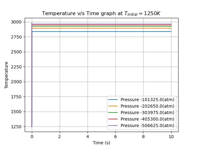
It can be seen that as the pressure increases the temperature also increases. From the ideal gas equation it is clear that as the pressure increases temperature also increases.
The ignition delay versus pressure graph is shown below:
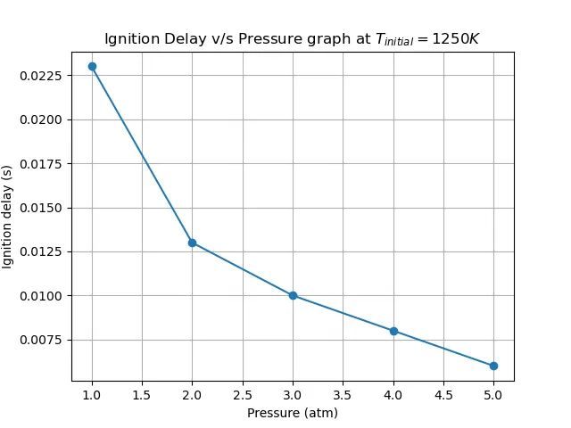
From this graph it can be seen that as the pressure increases the ignition delay also decreases. For a very high value of pressure the ignition delay can be further reduced.
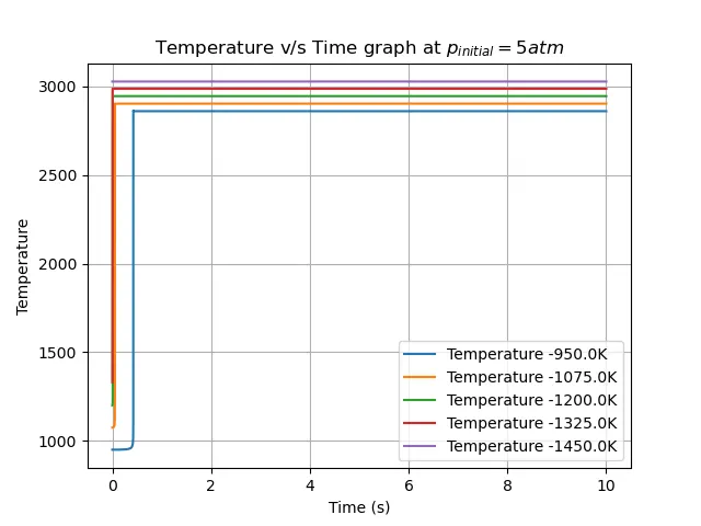
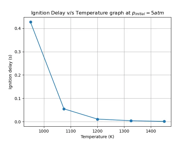
For analysing the effect of temperature variation on auto ignition temperature of methane air mixture, the pressure is kept at 5 atm and temperature is varied between 950 to 1450K. The temperature time graph is plotted for different values of initial temperature and also the ignition delay for different temperatures is also calculated. The codes and plots are shown below:
import cantera as ct
import matplotlib.pyplot as plt
import numpy as np


P = 5*ct.one_atm
ignition_delay =[]

T_min = 950 #K
T_max = 1450 #K
n = 5

T = np.linspace(T_min,T_max,n)

for j in range(0,len(T)):

	gas = ct.Solution('gri30.xml')
	gas.TPX = T[j], P,{'CH4':1,'O2':2,'N2':7.52}

	r =ct.IdealGasReactor(gas)

	sim = ct.ReactorNet([r])

	time = 0.00

	states = ct.SolutionArray(gas,extra=['time_in_ms','t'])

	Told = T[j]

	for k in range(10000):
		time = time +1e-3
		sim.advance(time)
		states.append(r.thermo.state,time_in_ms=time*1e-3,t=time)

		Tnew = states.T
		Tnew = Tnew[k-1]

		if ((Tnew-Told )>400):
			ignition_delay.append(time)

		Told = states.T
		Told = Told[k-1]


	plt.plot(states.t,states.T)
plt.xlabel('Time (s)')
plt.ylabel('Temperature')
plt.legend(['Temperature -' + str(h)+ 'K' for h  in T])
plt.title(r'Temperature v/s Time graph at $p_{initial} =  5 atm$')
plt.grid()
plt.savefig('Time-Tempatdifftemp.png')
plt.show()

plt.plot(T,ignition_delay,'o-')
plt.xlabel('Temperature (K)')
plt.ylabel('Ignition delay (s)')
plt.title(r'Ignition Delay v/s Temperature graph at $p_{initial} = 5 atm$')
plt.grid()
plt.savefig('igntiondelay_press.png')
plt.show()
The results are shown below:
In the second part of the study, molar concentrations of the given elements `H_2O`, `O_2` and `OH` with respect to the time is calculated for 1000K and 500K and the graphs are plotted. The program is shown below:
import cantera as ct
import matplotlib.pyplot as plt
import numpy as np


P = 5*ct.one_atm
ignition_delay =[]


T = 500 #K


gas = ct.Solution('gri30.xml')
gas.TPX = T, P,{'CH4':1,'O2':2,'N2':7.52}

r =ct.IdealGasReactor(gas)

sim = ct.ReactorNet([r])

time = 0.00

states = ct.SolutionArray(gas,extra=['time_in_ms','t'])

Told = T

for k in range(10000):

	time = time +1e-3
	sim.advance(time)
	states.append(r.thermo.state,time_in_ms=time*1e-3,t=time)

	Tnew = states.T
	Tnew = Tnew[k-1]

	if ((Tnew-Told )>400):

		ignition_delay.append(time)

	Told = states.T
	Told = Told[k-1]


plt.figure(figsize=(20,10))
plt.subplot(1,3,1)
plt.plot(states.t,states.X[:,gas.species_index('H2O')])
plt.xlabel('Time (s)')
plt.ylabel(r'$\chi_{H_2O}$')
plt.title(r'Mole fraction of $H_2O$')
plt.grid()

plt.subplot(1,3,2)
plt.plot(states.t,states.X[:,gas.species_index('O2')])
plt.xlabel('Time (s)')
plt.ylabel(r'$\chi_{O_2}$')
plt.title(r'Mole fraction of $O_2$')
plt.grid()

plt.subplot(1,3,3)
plt.plot(states.t,states.X[:,gas.species_index('OH')])
plt.xlabel('Time (s)')
plt.ylabel(r'$\chi_{OH}$')
plt.title(r'Mole fraction of $OH$')
plt.suptitle(r'Concentration of $H_2O$, $O_2$, $OH$ at T ='+ str(T) + 'K')
plt.grid()
plt.savefig('moleftraction'+ str(T)+ '.png')
plt.show()
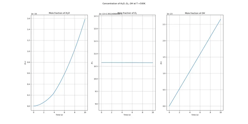
The results of the above codes are shown below. For an initial temperature of 500K, we can see that the mole fraction of `H_2O` is increasing as the reaction proceeds, since the temperature is not that high the `O_2` concentration almost remains the same and the `OH` concentration also increases. Even after 10 s the reaction dosent reach an equilibrium.
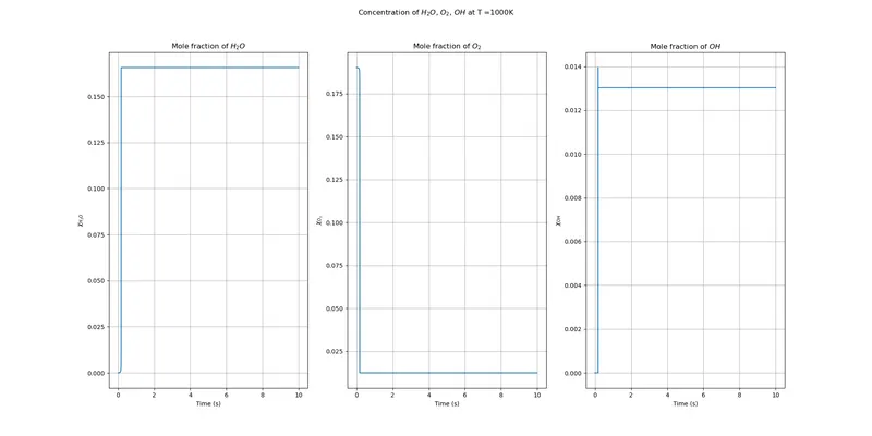
In the second case when the temperature is 1000K, the mole fraction of `H_2O` which is low at first steeply increases after autoignition and then the concentration reaches an equilibrium when the concentration doesn't vary with time. The mole fraction of `O_2` reduces with time and reaches an equilibrium and the mole fraction of `OH` also increases and reaches an equilibrium.
CONCLUSION
Autoignition analysis is carried out using python and cantera. It is seen that as the pressure is increased the ignition delay decreases, as the initial temperature increases the ignition delay also decreases.
For higher value of initial temperature, the equilibriumm temperature also increases, the case is same for higher value of chamber pressure. As the initial pressure is large the equilibrium temperature will be high.
When the temperature is 500 K the chemical reaction is not reaching a chemical equilibrium, but when the initial temperature is 1000 K after autoignition the mole fraction of `H_2O`, `O_2` and `OH` remains constant, which implies that chemicl equilibrium is reached.