Week 7 - Auto ignition using Cantera
#Aim:1.)To study variation of Auto ignition time of Methane for constant temperature 1250K and pressure wavering between 1 to 5 atm.
2.) To study variation of Auto ignition time of Methane for constant pressure 5 atm and temperature wavering between 950 K to 1450 K.
3.)To observe the rate of change of molar concentrations of the given elements "H2O, O2, OH" with respect to the time.
Introduction:
Autoignition occurs when a mixture of gases or vapors ignites spontaneously with no external ignition
source and after reaching a certain temperature, the autoignition temperature. The autoignition
temperature is not an intrinsic property of the gases or vapors but is the lowest temperature in a
system where the rate of heat evolved from the gases or vapors increases beyond the rate of heat loss
to the surroundings, resulting in ignition. The autoignition temperature of a mixture of gases or vapors is
affected by pressure,vessel shape and volume, surface activity, contaminants, flow rate, reaction rate,
droplet and mist formation, gravity, and reactant concentration.
-------------------------------------------------**************-----------------------------------------------
#Coding Approach:
1.)All required packages imported.
2.)Instance object 'gas' of Solution class created.
3.)All required variables defined.
4.)For each part ,a function is prepared.
5.)Inside each function ,gas parameters are set.
6.)Reactor object 'r' and ReactorNet object 'sim are defined.
7.)'sim' object is advanced with every time step,to find its value at each time step.
8.After getting results,they are plotted.
--------------------------------------------**********************-----------------------------------------
#Program for this complete challenge:
import cantera as ct
import matplotlib.pyplot as plt
import numpy as np

gas=ct.Solution('gri30.xml')												#A instance object (gas) of Solution class created
T=np.arange(950,1550,100)													#Temperature array defined
p_list=[1,2,3,4,5]															#Pressure list defined
p=np.array(p_list)															#Pressure array defined
P=p*101325

P_legend_list=['1 atm','2 atm','3 atm','4 atm','5 atm']
T_legend_list=['950 K','1050 K','1150 K','1250 K','1350 K','1450 K']

species_dict={'CH4':1,'O2':2,'N2':7.52}


def f_cons_temp(species_dict,P,T=1250):

	"""
		Function takes constant temperature 1250 K ,  pressure values from P and species composition for combustion

		Return states of gas object,Temperature before Autoignition and Ignition delay time
	"""
	gas.TPX=T,P,species_dict
	r=ct.IdealGasReactor(gas)							#Reactor object r from class  IdealGasConstPressureReactor defined,it contains gas object
	sim=ct.ReactorNet([r])								#Object sim from class ReactorNet defined having reactor r

	time=0.0											#Initial time set to zero
	states=ct.SolutionArray(gas)						#Solution array defined having all properties of gas object
	total_time=[]
	time_igni_delay=[]
	T_igni_values=[]
	for i in range(10000):
		time=time+1e-3
		sim.advance(time)								#advance() method useed to change state of object w.r.t time (t)
		states.append(r.thermo.state)
		T_comb_temp=states.T
		total_time.append(time)


	T_igni_values=T_comb_temp[T_comb_temp<T+400]		#Ignition delay temperature=Initial Temp +400 ,T_igni_values storing temperature till ignition delay time.
	time_igni_delay=total_time[0:len(T_igni_values)]

	x=(states.T,T_igni_values,time_igni_delay)

	return x


for i in range(len(P)):
	Value_of_func_cons_Temp=f_cons_temp(species_dict,P[i])
	plt.plot(Value_of_func_cons_Temp[2],Value_of_func_cons_Temp[1],label=P_legend_list[i])
	plt.xlabel('Ignition Delay time (in seconds)')
	plt.ylabel('Temperature (in Kelvin)')
	plt.title('Plot showing change in Ignition Delay time with change in pressure inside reactor')
	plt.legend(loc="upper right")

plt.show()


def f_cons_pres(species_dict,T,P=ct.one_atm*5):

	"""
		Function takes constant  pressure 5 atm ,  temperature values from T list and species composition for combustion

		Return states of gas object,Temperature before Autoignition and Ignition delay time
	"""
	gas.TPX=T,P,species_dict
	r=ct.IdealGasReactor(gas)
	sim=ct.ReactorNet([r])
	time=0.0
	states=ct.SolutionArray(gas)
	total_time=[]
	time_igni_delay=[]
	T_igni_values=[]
	for i in range(100000):
		time=time+1e-4
		sim.advance(time)
		states.append(r.thermo.state)
		T_comb_temp=states.T

		total_time.append(time)


	T_igni_values=T_comb_temp[T_comb_temp<T+400]
	time_igni_delay=total_time[0:len(T_igni_values)]


	x=(states.T,T_igni_values,time_igni_delay)

	return x


for i in range(len(T)):
	Value_of_func_cons_Pres=f_cons_pres(species_dict,T[i])
	print(Value_of_func_cons_Pres[2])
	plt.plot(Value_of_func_cons_Pres[2],Value_of_func_cons_Pres[1],label=T_legend_list[i])
	plt.legend(loc="upper right")
	plt.xlabel('Ignition Delay time (in seconds)')
	plt.ylabel('Temperature (in Kelvin)')
	plt.title('Plot showing change in Ignition Delay time with change in initial Temperature inside reactor')

plt.show()


def f_cons_P_T1000(species_dict,P=101325*5,T=1000):

	"""
		Function takes constant  pressure 5 bar ,  temperature 1000 K and species composition for combustion

		Return states of gas object, its Temperature,Total time,Temperature before Autoignition and Ignition delay time
	"""
	gas.TPX=T,P,species_dict
	r=ct.IdealGasReactor(gas)
	sim=ct.ReactorNet([r])
	time=0.0
	states=ct.SolutionArray(gas)
	total_time=[]
	time_igni_delay=[]
	T_igni_values=[]
	for i in range(10000):
		time=time+1e-3
		sim.advance(time)
		states.append(r.thermo.state)
		T_comb_temp=states.T
		total_time.append(time)


	T_igni_values=T_comb_temp[T_comb_temp<T+400]
	time_igni_delay=total_time[0:len(T_igni_values)]


	x=(states,states.T,T_igni_values,time_igni_delay,total_time)

	return x


Value_of_func_cons_P_T1000=f_cons_P_T1000(species_dict)


Val_of_molar_conc_H2O=Value_of_func_cons_P_T1000[0].X[:,gas.species_index('H2O')]
Val_of_molar_conc_O2=Value_of_func_cons_P_T1000[0].X[:,gas.species_index('O2')]
Val_of_molar_conc_OH=Value_of_func_cons_P_T1000[0].X[:,gas.species_index('OH')]
plt.figure(3)
plt.plot(Value_of_func_cons_P_T1000[4],Val_of_molar_conc_H2O,label='H2O')
plt.legend(loc="upper right")
plt.xlabel('Total time (in seconds)')
plt.ylabel('Molar concentration of H2O')
plt.title('Plot showing variation in H2O Molar conc. w.r.t Time with Initial Temp=1000k and Pressure=5 bar inside reactor')
plt.figure(4)
plt.plot(Value_of_func_cons_P_T1000[4],Val_of_molar_conc_O2,label='O2')
plt.legend(loc="upper right")
plt.xlabel('Total time (in seconds)')
plt.ylabel('Molar concentration of O2')
plt.title('Plot showing variation in O2 Molar conc. w.r.t Time with Initial Temp=1000k and Pressure=5 bar inside reactor')
plt.figure(5)
plt.plot(Value_of_func_cons_P_T1000[4],Val_of_molar_conc_OH,label='OH')
plt.legend(loc="upper right")
plt.xlabel('Total time (in seconds)')
plt.ylabel('Molar concentration of OH')
plt.title('Plot showing variation in OH Molar conc. w.r.t Time with Initial Temp=1000k and Pressure=5 bar inside reactor')
print('Molar conc of H2O {0} ,\nMolar conc of O2\n {1} ,\nMolar conc of OH\n {2}'.format(Val_of_molar_conc_H2O,Val_of_molar_conc_O2,Val_of_molar_conc_OH))

plt.show()


def f_cons_P_T500(species_dict,P=101325*5,T=500):

	"""
		Function takes constant  pressure 5 bar ,  temperature 500 K and species composition for combustion

		Return states of gas object, its Temperature,Total time,Temperature before Autoignition and Ignition delay time
	"""
	gas.TPX=T,P,species_dict
	r=ct.IdealGasReactor(gas)
	sim=ct.ReactorNet([r])
	time=0.0
	states=ct.SolutionArray(gas)
	total_time=[]
	time_igni_delay=[]
	T_igni_values=[]
	for i in range(10000):
		time=time+1e-3
		sim.advance(time)
		states.append(r.thermo.state)
		T_comb_temp=states.T
		total_time.append(time)


	T_igni_values=T_comb_temp[T_comb_temp<T+400]
	time_igni_delay=total_time[0:len(T_igni_values)]


	x=(states,states.T,T_igni_values,time_igni_delay,total_time)

	return x


Value_of_func_cons_P_T500=f_cons_P_T500(species_dict)
Val_of_molar_conc_H2O=Value_of_func_cons_P_T500[0].X[:,gas.species_index('H2O')]
Val_of_molar_conc_O2=Value_of_func_cons_P_T500[0].X[:,gas.species_index('O2')]
Val_of_molar_conc_OH=Value_of_func_cons_P_T500[0].X[:,gas.species_index('OH')]


plt.figure(6)
plt.plot(Value_of_func_cons_P_T500[4],Val_of_molar_conc_H2O,label='H2O')
plt.xlabel('Total time (in seconds)')
plt.ylabel('Molar concentration of H2O')
plt.legend(loc="upper right")
plt.title('Plot showing variation in H2O Molar conc. w.r.t Time with Initial Temp=1000k and Pressure=5 bar inside reactor')
plt.figure(7)
plt.plot(Value_of_func_cons_P_T500[4],Val_of_molar_conc_O2,label='O2')
plt.xlabel('Total time (in seconds)')
plt.ylabel('Molar concentration of O2')
plt.title('Plot showing variation in O2 Molar conc. w.r.t Time with Initial Temp=1000k and Pressure=5 bar inside reactor')
plt.legend(loc="upper right")
plt.figure(8)
plt.plot(Value_of_func_cons_P_T500[4],Val_of_molar_conc_OH,label='OH')
plt.legend(loc="upper right")
plt.xlabel('Total time (in seconds)')
plt.ylabel('Molar concentration of OH')
plt.title('Plot showing variation in OH Molar conc. w.r.t Time with Initial Temp=500k and Pressure=5 bar inside reactor')

print('Molar conc of H2O {0} ,\nMolar conc of O2\n {1} ,\nMolar conc of OH\n {2}'.format(Val_of_molar_conc_H2O,Val_of_molar_conc_O2,Val_of_molar_conc_OH))

plt.show()
Part-1
Case-1:
In the first case ,Initial temperature is 1250 K and pressure varying from 1 to 5 atm.
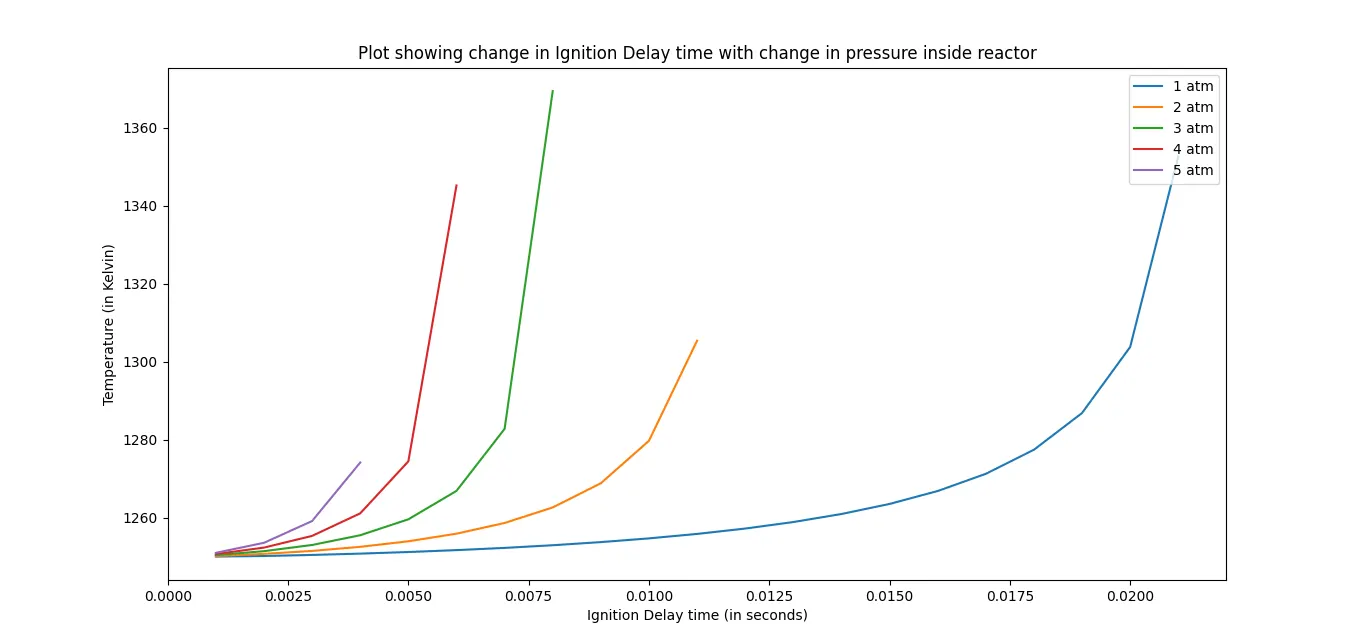
From the plot we can see that with the increase in pressure for same initial temperature ,Ignition delay time decreases.
-------------------------------------------************************----------------------------------------
Case-2:
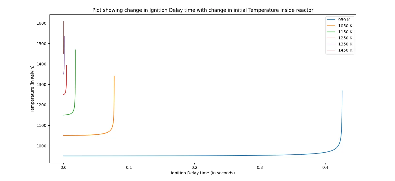
From the plot we can say that,for same pressure and with increase in temperature ,ignition delay time decreases.
Part-2
Case-1:When Temperature is 1000K and pressure 5 bar.
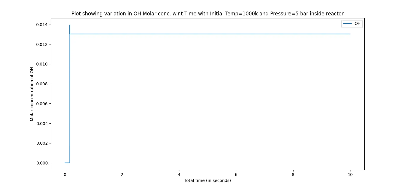
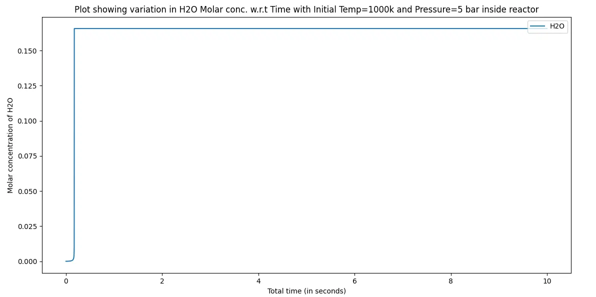
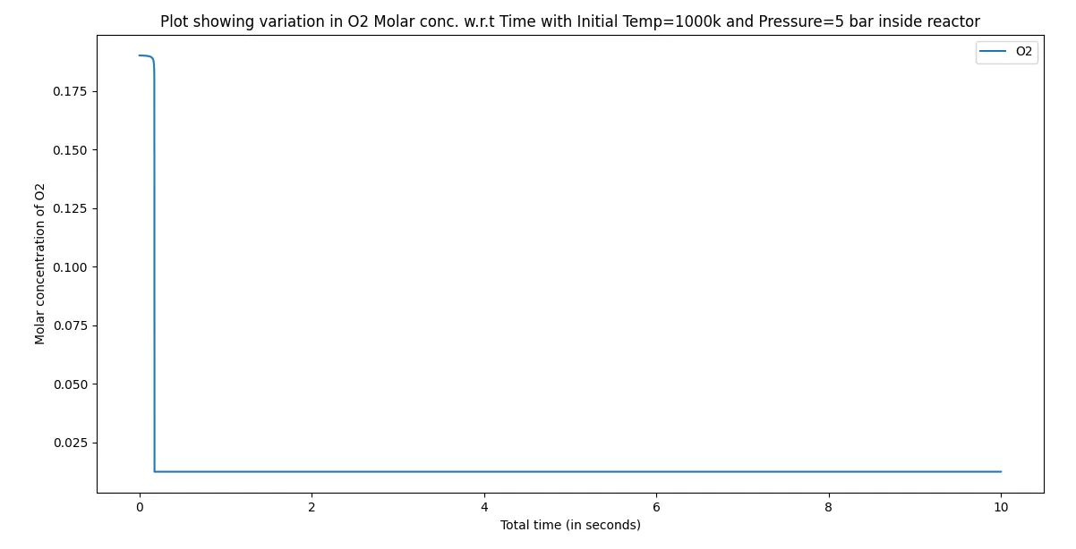
As the plot indicates,when the combustion takes place ,O2 concentration will decrease and H20 and OH will be produced in products,so their concentration increases.
------------------------------------------*********************------------------------------------
Case-2: When Temperature is 500K and pressure 5 bar.
At this temperature and pressure there will not be any combustion ,it does not matter for how much time we run the simulation.
Below plots indicate the same.
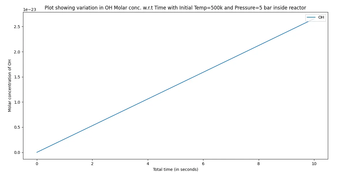
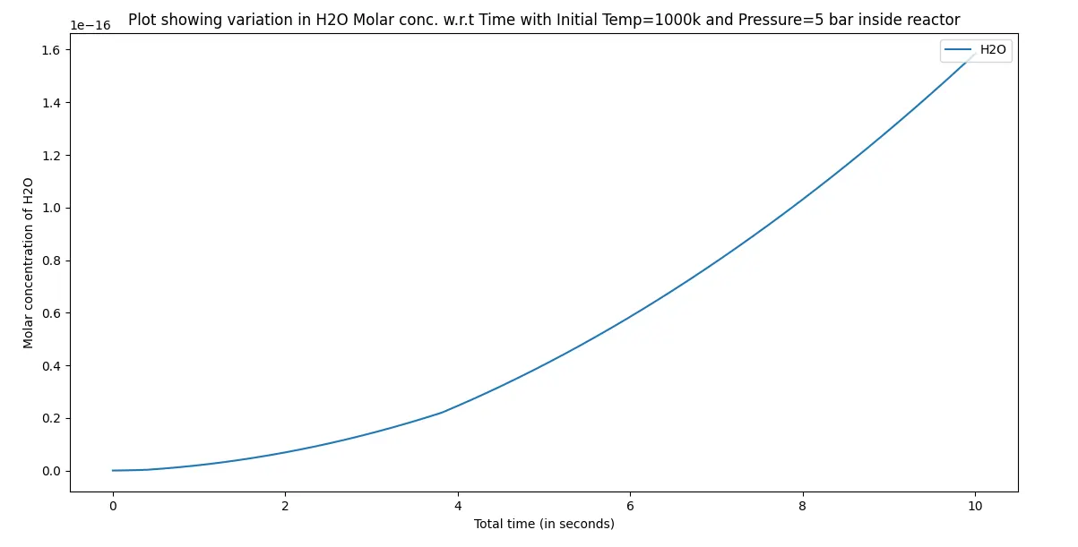
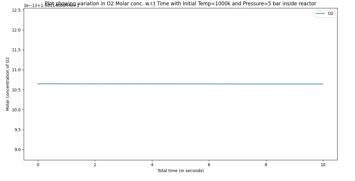
O2 concentration is constant this means there is no combustion.H2O and OH concentration increase little bit that is negligible(equivalent to zero).