Auto ignition using Cantera
AIM
The aim of this challenge is to simulate the auto ignition temperature for methane
OBJECTIVES
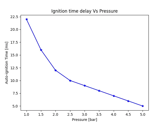
- Variation of Auto Ignition time of Methane with a constant temperature of 1250K and pressure varying from 1 to 5 atm.
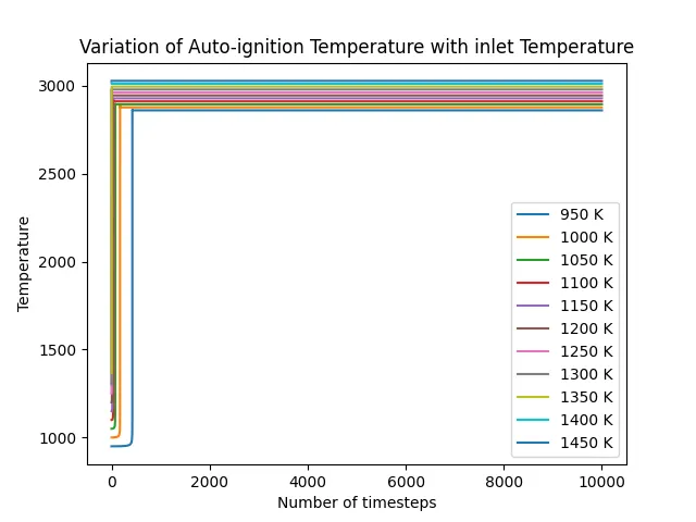
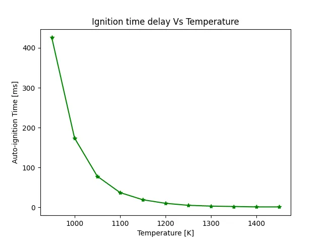
- Variation of Auto Ignition time of Methane with a constant pressure of 5 atm and temperature varying from 950K to 1450K.
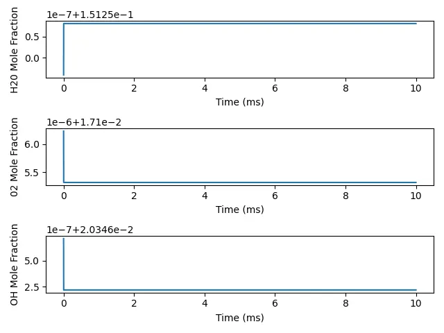
- Rate of change of molar concentrations of the given elements "H2O, O2, OH" with respect to the time
REACTORS NETWORK IN CANTERA
A Cantera Reactor() represents the simplest form of a chemically reacting system. It corresponds to an extensive thermodynamic control volume VV, in which all state variables are homogeneously distributed. The system is generally unsteady — that is, all states are functions of time. In particular, transient state changes due to chemical reactions are possible. However, thermodynamic (but not chemical) equilibrium is assumed to be present throughout the reactor at all instants of time.
Reactors can interact with the surrounding environment in multiple ways:
-
Expansion/compression work: By moving the walls of the reactor, its volume can be changed and expansion or compression work can be done by or on the reactor.
-
Heat transfer: An arbitrary heat transfer rate can be defined to cross the boundaries of the reactor.
-
Mass transfer: The reactor can have multiple inlets and outlets. For the inlets, arbitrary states can be defined. Fluid with the current state of the reactor exits the reactor at the outlets.
-
Surface interaction: One or multiple walls can influence the chemical reactions in the reactor. This is not just restricted to catalytic reactions, but mass transfer between the surface and the fluid can also be modeled.
All of these interactions do not have to be constant, but can vary as a function of time or state. For example, heat transfer can be described as a function of the temperature difference between the reactor and the environment, or the wall movement can be modeled depending on the pressure difference. Interactions of the reactor with the environment are defined on one or more walls, inlets, and outlets.
In addition to single reactors, Cantera is also able to interconnect reactors into a Reactor Network. Each reactor in a network may be connected so that the contents of one reactor flow into another. Reactors may also be in contact with one another or the environment via walls that conduct heat or move to do work.
Governing Equations for Single Reactors
The state variables for Cantera’s general reactor model are
-
mm, the mass of the reactor’s contents (in kg)
-
VV, the reactor volume (in m3) (not a state variable for
ConstPressureReactor()andIdealGasConstPressureReactor()) -
A state variable describing the energy of the system, depending on the configuration (see Energy Conservation for further explanation):
-
General
Reactor(): UU, the total internal energy of the reactors contents (in J) -
ConstPressureReactor(): HH, the total enthalpy of the reactors contents (in J) -
IdealGasReactor()andIdealGasConstPressureReactor(): TT, the temperature (in K)
-
-
Y_kYk, the mass fractions for each species (dimensionless)
Mass Conservation
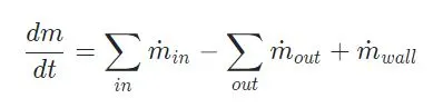
The total mass of the reactor’s contents changes as a result of flow through the reactor’s inlets and outlets, and production of homogeneous phase species on the reactor walls:
Species Conservation
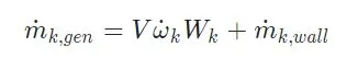
The rate at which species kk is generated through homogeneous phase reactions is V dot{omega}_k W_kVω˙kWk, and the total rate at which species kk is generated is:
The rate of change in the mass of each species is:

Expanding the derivative on the left hand side and substituting the equation for dm/dtdm/dt, the equation for each homogeneous phase species is:

Reactor Volume
The reactor volume changes as a function of time due to the motion of one or more walls:
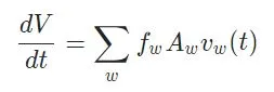
where f_w = pm 1fw=±1 indicates the facing of the wall (whether moving the wall increases or decreases the volume of the reactor), A_wAw is the surface area of the wall, and v_w(t)vw(t) is the velocity of the wall as a function of time.
For the ConstPressureReactor() and IdealGasConstPressureReactor(), the volume is not a state variable, but instead takes on whatever value is consistent with holding the pressure constant.
Energy Conservation
The solution of the energy equation can be enabled or disabled by changing the energy_enabled flag. It is enabled by default.
The implemented formulation of the energy equation depends on which reactor model is used.
Standard Reactor
The equation for the total internal energy is found by writing the first law for an open system:

Constant Pressure Reactor
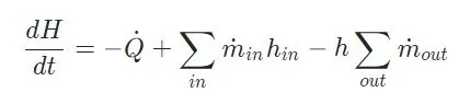
For this reactor model, the pressure is held constant. The volume is not a state variable, but instead takes on whatever value is consistent with holding the pressure constant. The total enthalpy replaces the total internal energy as a state variable. Using the definition of the total enthalpy:
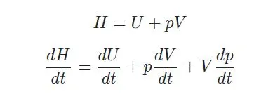
Noting that dp/dt = 0dp/dt=0 and substituting into the energy equation yields:
Ideal Gas Reactor
In case of the Ideal Gas Reactor Model, the reactor temperature TT is used instead of the total internal energy UU as a state variable. For an ideal gas, we can rewrite the total internal energy in terms of the mass fractions and temperature:
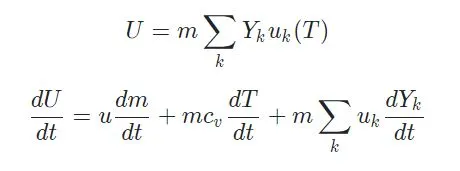
Substituting the corresponding derivatives yields an equation for the temperature:

While this form of the energy equation is somewhat more complicated, it significantly reduces the cost of evaluating the system Jacobian, since the derivatives of the species equations are taken at constant temperature instead of constant internal energy.
Ideal Gas Constant Pressure Reactor
As for the Ideal Gas Reactor, we replace the total enthalpy as a state variable with the temperature by writing the total enthalpy in terms of the mass fractions and temperature:
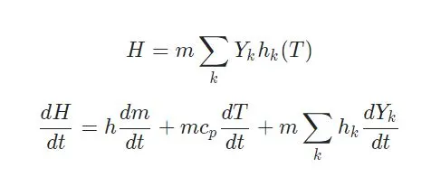
Substituting the corresponding derivatives yields an equation for the temperature:

import matplotlib.pyplot as plt
import cantera as ct
import numpy as np


gas = ct.Solution('gri30.xml')
pressure = np.linspace(1,5,9)
T_int = 1250
time_start = 0.0
time_end = 10.0
time_step = 1e-3
n = int((time_end - time_start)/time_step)
t_autoI_P = []
states1 = []

for i in pressure:
	gas.TPX = T_int, i*101325,{'CH4':1,'O2':2,'N2':7.52}
	T_autoI = 0
	t_autoI = 0
	time = 0
	r = ct.IdealGasReactor(gas)
	sim = ct.ReactorNet([r])
	states = ct.SolutionArray(gas, extra=['time_in_ms','t'])
	print('{:10s} {:10s} {:10s}'.format('t [s]','T [K]','P [Pa]'))

	for n in range(n):
		time += 1e-3
		sim.advance(time)
		states.append(r.thermo.state,time_in_ms = time*1e3,t = time)
		print('{:10.3e} {:10.3f} {:10.3f} '.format(sim.time, r.T, r.thermo.P))
	states1.append(states.T)

	for i in range(n):
		T_error = states.T[i] - T_int - 400
		if T_error > 0:
			T_autoI = states.T[i]
			t_autoI = states.time_in_ms[i]
			break
	t_autoI_P.append(t_autoI)


states1 = np.array(states1)
for k in range(len(pressure)):
	plt.figure(1)
	plt.plot(states1[k])
	plt.xlabel('Number of timesteps')
	plt.ylabel('Temperature')
	plt.title('Variation of Auto-ignition Temperature with inlet Pressure')
	plt.legend(['1 Bar','1.5 Bar', '2 Bar', '2.5 Bar','3 Bar','3.5 Bar', '4 Bar', '4.5 Bar', '5 Bar'])

plt.figure(2)
plt.plot(pressure,t_autoI_P,'b-*')
plt.xlabel('Pressure [bar]')
plt.ylabel('Auto-ignition Time [ms]')
plt.title('Ignition time delay Vs Pressure')
plt.show()
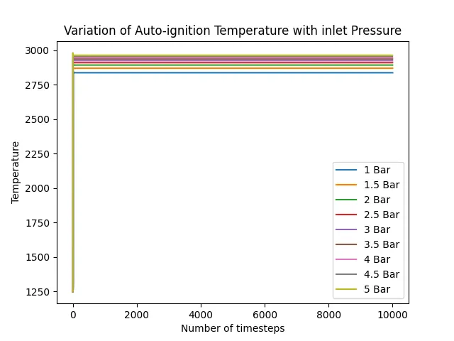
The code starts with necessary libraries and then the gas object is defined from the concepts of object oriented programming. The temperature of gas is assumed to be at 1250 K and then we write the start time and end time parameters in the subsequent lines of the program. We are saying the program to run the solution for 10 seconds with a time step of 1ms or 1e-3 seconds. Now since the pressure is to be varied from 1 bar to 5 bar, the linspace command defines 9 values of pressure. The for loop is used to execute the reactor network operations. Now when we define r, sim and states variables with the following statements, from these objects we are calling the respective classes of the created objects. Then we are appending the states object by defining the convergence loop of error. The results are then plotted as shown below
import matplotlib.pyplot as plt
import numpy as np
import cantera as ct

gas = ct.Solution('gri30.xml')
Temperature = np.linspace(950,1450,11)
time_start =0.0
time_end = 10.0
time_step =1e-3
n = int((time_end - time_start)/time_step)
t_autoI_T = []
states1 = []

for i in Temperature:
	gas.TPX = i, 5*101325, {'CH4':1,'O2':2,'N2':7.52}
	T_autoI = 0
	t_autoI = 0
	time = 0
	r = ct.IdealGasReactor(gas)
	sim = ct.ReactorNet([r])
	states = ct.SolutionArray(gas, extra=['time_in_ms','t'])
	print('{:10s} {:10s} {:10s}'.format('t [s]','T [K]','P [Pa]'))

	for j in range(n):
		time += 1e-3
		sim.advance(time)
		states.append(r.thermo.state,time_in_ms= time*1e3, t = time)
		print('{:10.3e} {:10.3f} {:10.3f} '.format(sim.time, r.T, r.thermo.P))
	states1.append(states.T)

	for j in range(n):
		T_error = states.T[j] - i - 400
		if T_error > 0:
			T_autoI = states.T[j]
			t_autoI = states.time_in_ms[j]
			break
	t_autoI_T.append(t_autoI)

states1 = np.array(states1)
for k in range(len(Temperature)):
	plt.figure(1)
	plt.plot(states1[k])
	plt.xlabel('Number of timesteps')
	plt.ylabel('Temperature')
	plt.title('Variation of Auto-ignition Temperature with inlet Temperature')
	plt.legend(['950 K','1000 K', '1050 K', '1100 K','1150 K','1200 K', '1250 K', '1300 K', '1350 K', '1400 K','1450 K'])

plt.figure(2)
plt.plot(Temperature,t_autoI_T,'g-*')
plt.xlabel('Temperature [K]')
plt.ylabel('Auto-ignition Time [ms]')
plt.title('Ignition time delay Vs Temperature')
plt.show()
The code starts with necessary libraries and then the gas object is defined from the concepts of object oriented programming. The pressure of gas is assumed to be at 1.01325 bar and then we write the start time and end time parameters in the subsequent lines of the program. We are saying the program to run the solution for 10 seconds with a time step of 1ms or 1e-3 seconds. Now since the temperature is to be varied from 950 K bar to 1450 K, the linspace command defines 11 values of pressure. The for loop is used to execute the reactor network operations. Now when we define r, sim and states variables with the following statements, from these objects we are calling the respective classes of the created objects. Then we are appending the states object by defining the convergence loop of error. The results are then plotted as shown below
PLOTS FOR CODE
CODE FOR AUTO IGNITION WITH VARYING MOLAR CONCENTRATION
import matplotlib.pyplot as plt
import cantera as ct
import numpy as np


gas = ct.Solution('gri30.xml')
Temperature = np.linspace(950,1450,11)
time_start =0.0
time_end = 10.0
time_step =1e-3
n = int((time_end - time_start)/time_step)
t_autoI_T = []
states1 = []
for i in Temperature:
	gas.TPX = i, 5*101325, {'CH4':1,'O2':2,'N2':7.52}
	T_autol = 0
	t_autoI = 0
	time = 0
	r = ct.IdealGasReactor(gas)
	sim = ct.ReactorNet([r])
	states = ct.SolutionArray(gas, extra=['time_in_ms','t'])
	print('{:10s} {:10s} {:10s}'.format('t [s]','T [K]','P [Pa]'))
	for j in range(n):
		time += 1e-3
		sim.advance(time)
		states.append(r.thermo.state,time_in_ms= time*1e3, t=time)
		print('{:10.3e} {:10.3f} {:10.3f} '.format(sim.time, r.T, r.thermo.P))
	states1.append(states.T)
	for j in range(n):
		T_error = states.T[j] - i -400
		if T_error > 0:
			T_autol = states.T[j]
			t_autol = states.time_in_ms[j]
			break
		t_autoI_T.append(t_autoI)
plt.figure(1)
plt.subplot(3, 1, 1)
plt.plot(states.t, states.X[:,gas.species_index('H2O')])
plt.xlabel('Time (ms)')
plt.ylabel('H20 Mole Fraction')
plt.subplot(3, 1, 2)
plt.plot(states.t, states.X[:,gas.species_index('O2')])
plt.xlabel('Time (ms)')
plt.ylabel('02 Mole Fraction')
plt.subplot(3, 1, 3)
plt.plot(states.t, states.X[:,gas.species_index('OH')])
plt.xlabel('Time (ms)')
plt.ylabel('OH Mole Fraction')
plt.tight_layout()
plt.show()
The code starts with necessary libraries and then the gas object is defined from the concepts of object oriented programming. The pressure of gas is assumed to be at 1.01325 bar and then we write the start time and end time parameters in the subsequent lines of the program. We are saying the program to run the solution for 10 seconds with a time step of 1ms or 1e-3 seconds. Now since the temperature is to be varied from 950 K bar to 1450 K, the linspace command defines 11 values of pressure. The for loop is used to execute the reactor network operations. Now when we define r, sim and states variables with the following statements, from these objects we are calling the respective classes of the created objects. Then we are appending the states object by defining the convergence loop of error. The results are then plotted as shown below for the concentration of molar of species for respective products of combustion for methane.
PLOT FOR CODE
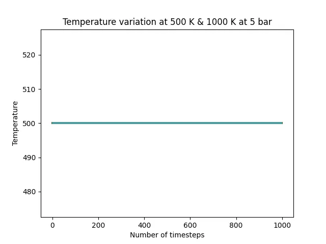
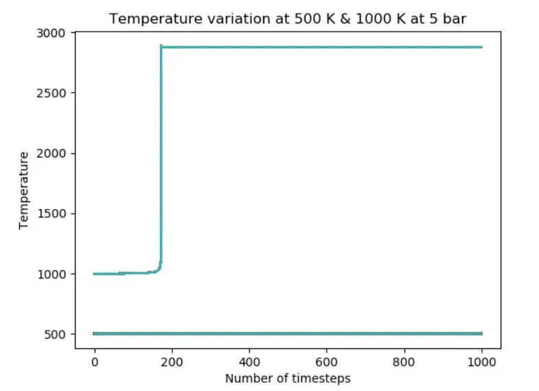
AUTO IGNITION FOR TEMPERATURE OF 500 K AND 1000K
import matplotlib.pyplot as plt
import cantera as ct
import numpy as np

gas = ct.Solution('gri30.xml')
Temperature = [500,1000]
states1 = []

for i in Temperature:
	gas.TPX = i, 5*101325, {'CH4':1, 'O2':2,'N2':7.52}
	r =ct.IdealGasReactor(gas)
	sim = ct.ReactorNet([r])
	time = 0.0
	states = ct.SolutionArray(gas)

	for n in range(1000):
		time += 1e-3
		sim.advance(time)
		states.append(r.thermo.state)

states1 = np.array(states.T)
for k in range(1000):
		plt.figure(1)
		plt.plot(states1)
		plt.xlabel('Number of timesteps')
		plt.ylabel('Temperature')
		plt.title('Temperature variation at 500 K & 1000 K at 5 bar')
		plt.show()
PLOT FOR CODE
CONCLUSION
- Variation of Auto Ignition time of Methane with a constant temperature of 1250K and pressure varying from 1 to 5 atm was examined
- Variation of Auto Ignition time of Methane with a constant pressure of 5 atm and temperature varying from 950K to 1450K. This study was conducted in the second case of the code
- Rate of change of molar concentrations of the given elements "H2O, O2, OH" with respect to the time was concluded
- The effect of temperature for 500 K and 1000 K is plotted which shows the auto ignition for only 1000 K.