Week 7 - Auto ignition using Cantera

Aim:

to simulate the Auto Ignition Time for Methane under the following conditions, (simulation time = 10 secs)

• Plot the variation of Auto Ignition time of Methane with a constant temperature of 1250K and pressure varying from 1 to 5 atm.
• Plot the variation of Auto Ignition time of Methane with a constant pressure of 5 atm and temperature varying from 950K to 1450K.

PART II

Further, observe and print the rate of change of molar concentrations of the given elements "H2O, O2, OH" with respect to the time, (simulation time = 10 secs)

Explain the behavior of the graph for 2 cases,

• When Temperature is 1000K and pressure 5 bar
• When Temperature is 500K and pressure 5 bar

variation of autoiginition time with initial temparature:-

import cantera as ct
import numpy as np
import matplotlib.pyplot as plt

gas = ct.Solution('gri30.xml')
P = 5*101325
t_start = 950
t_end = 1450
iginition_delay = []
a = 0
temp = np.linspace(t_start,t_end,5)
sim_time = 10000

for T in temp:
gas.TPX = T,P,{'CH4':1,'O2':2,'N2':7.52}
r = ct.IdealGasReactor(gas)
sim = ct.ReactorNet([r])
time = 0.0
T_old = T
a = 0
states = ct.SolutionArray(gas,extra = ['time_in_ms','t'])
for i in range(sim_time):
time += 1e-4
sim.advance(time)
states.append(r.thermo.state,time_in_ms = time*1e-3,t = time)
T_new = states.T
T_new = T_new[i]
if ((T_new-T_old)>=400 and a==0):
iginition_delay.append(time)
a = a+1

plt.figure(1)
plt.plot('states.time_in_ms,states.T')
plt.xlabel('time')
plt.ylabel('temparature')

plt.figure(2)
plt.plot(temp,iginition_delay ,'-o')
plt.xlabel('temparature')
plt.ylabel('iginition delay')
plt.show()

plots:

result:

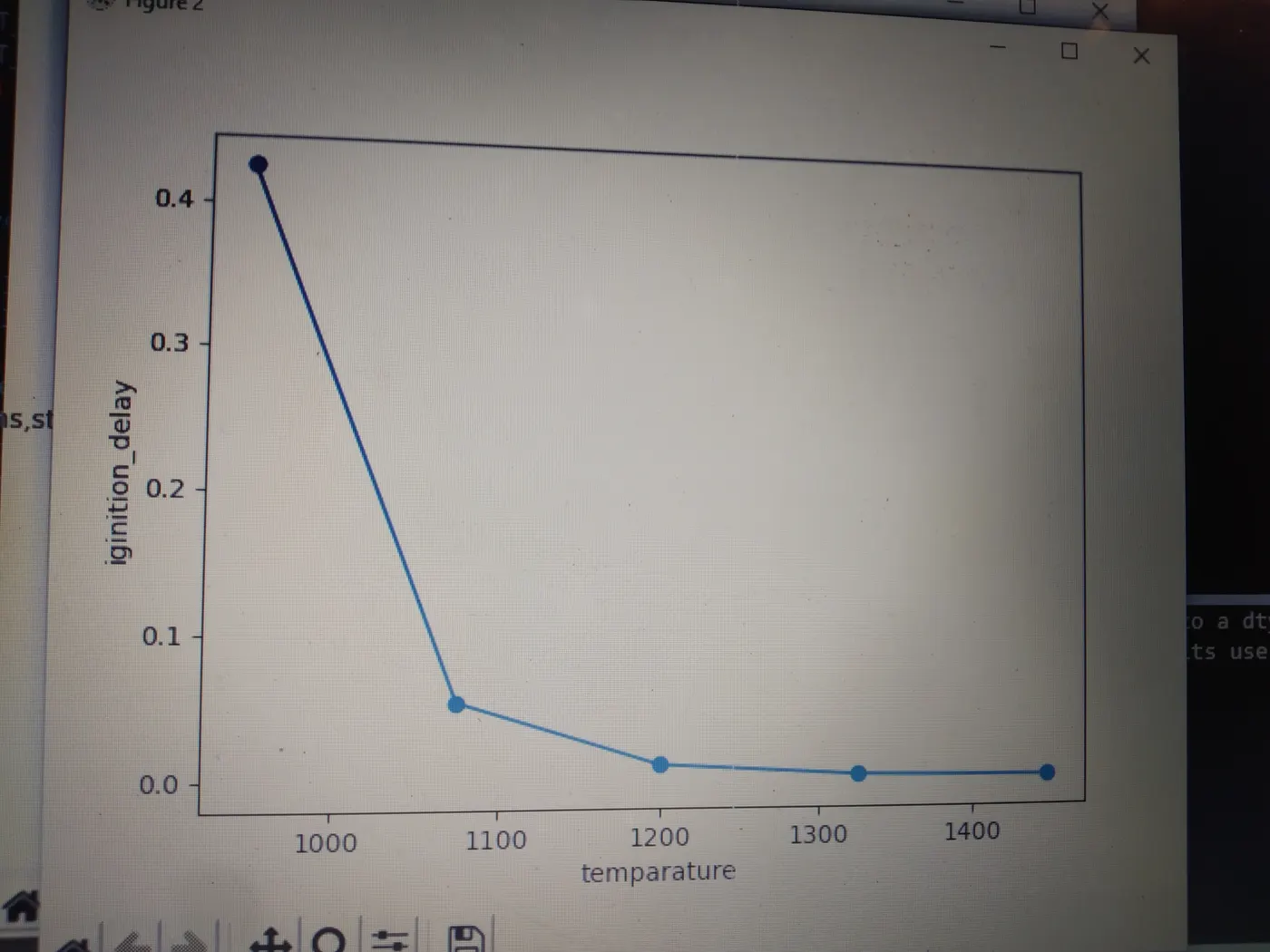
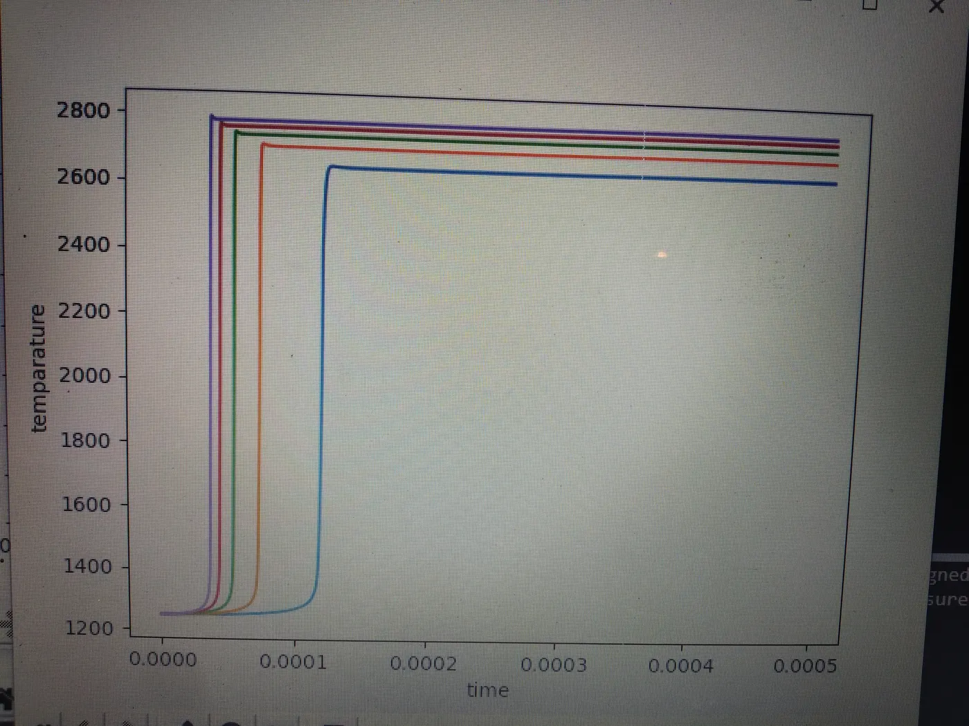
plot shows ignition delay with respective to delay time ,here we can say that for the higher tempatarures ignition delay time is less than milli seonds.

and for the lower tempatarures ignition delay time is 0.4 secs

from this we can say that iginition delay is sensitive to temparature

variation of autoiginition time with initial pressure:-

import cantera as ct
import numpy as np
import matplotlib.pyplot as plt

gas = ct.Solution('gri30.xml')
T = 1250
P_start = 1*10132
P_end = 5*10132
iginition_delay = []
a = 0
pressure = np.linspace(P_start,P_end,5)
sim_time = 5000

for P in pressure:
gas.TPX = T,P,{'CH4':1,'O2':2,'N2':7.52}
r = ct.IdealGasReactor(gas)
sim = ct.ReactorNet([r])
time = 0.0
T_old = T
a = 0
states = ct.SolutionArray(gas,extra = ['time_in_ms','t'])
for i in range(sim_time):
time += 1e-4
sim.advance(time)
states.append(r.thermo.state,time_in_ms = time*1e-3,t = time)
T_new = states.T
T_new = T_new[i]
if ((T_new-T_old)>=400 and a==0):
iginition_delay.append(time)
a = a+1

plt.figure(1)
plt.plot(states.time_in_ms,states.T)
plt.xlabel('time')
plt.ylabel('temparature')

plt.figure(2)
plt.plot(pressure,iginition_delay,'-o')
plt.xlabel('pressure')
plt.ylabel('iginition_delay')
plt.show()

plots:

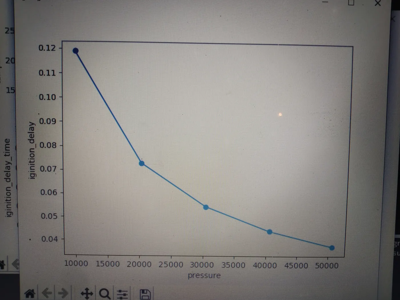
result:

concentartion of elements with time at different temparatures:-

import sys

import cantera as ct
import numpy as np
import matplotlib.pyplot as plt

gas = ct.Solution('gri30.xml')
temp = [500,1000]
P = 5*101325
sim_time = 10000

for T in temp:

gas.TPX = T,P,{'CH4':1,'O2':2,'N2':7.52}

r = ct.IdealGasReactor(gas)
sim = ct.ReactorNet([r])
T_old = T
time = 0
states = ct.SolutionArray(gas,extra = ['time_in_ms','t'])

for i in range(sim_time):
time += 1e-3
sim.advance(time)
states.append(r.thermo.state,time_in_ms = time*1e-3,t = time)

plt.subplot(3,1,1)
plt.title('Molar concentration vs Time')
plt.plot(states.t,states.X[:,gas.species_index('H2O')],'r')
plt.xlabel('time')
plt.ylabel('O2')

plt.subplot(3,1,2)
plt.plot(states.t,states.X[:,gas.species_index('O2')],'r')
plt.xlabel('time')
plt.ylabel('O2')

plt.subplot(3,1,3)
plt.plot(states.t,states.X[:,gas.species_index('OH')],'r')
plt.xlabel('time')
plt.ylabel('OH')
plt.show()

result:

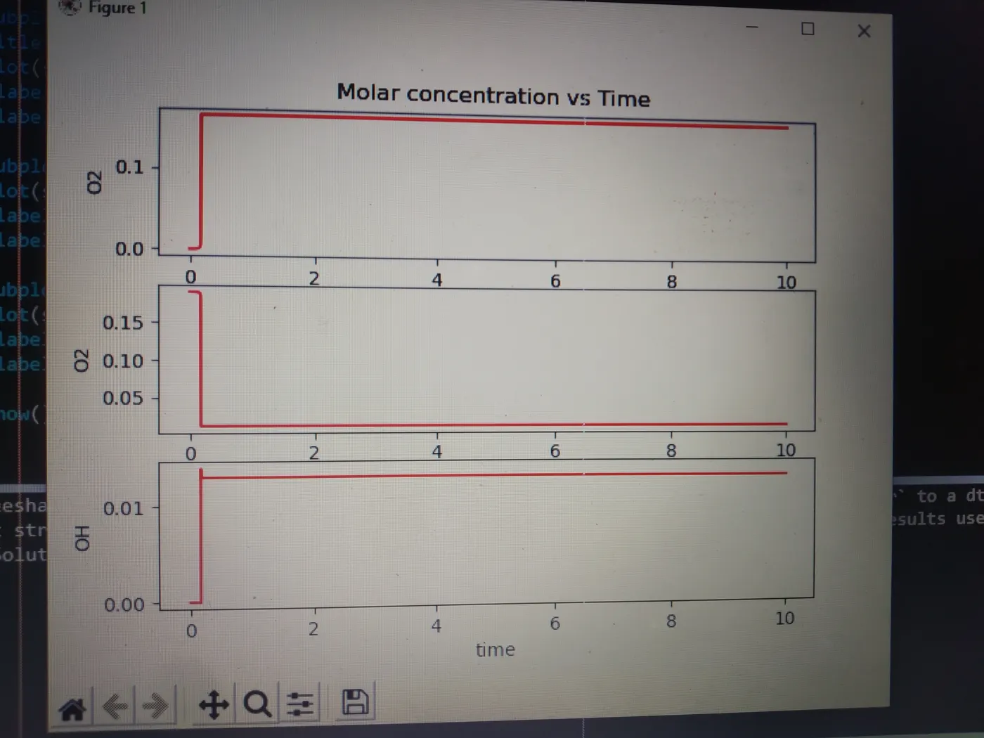
from the graph sudden spike represent the auto ignition with ignition delay

h20 mole fraction, it is increased and stabled throughout the simulation time

02 mole fraction, it is decreased and maintained stability

0h mole fraction, it is increased and stabled throughout the simulation time