Auto ignition using Cantera

Objectives:

1. Plot the effect of pressure on auto ignition time, with constant inlet temperature
2. Plot the effect of inlet temperature on auto ignition time, with constant pressure
3. Plot the rate of change of molar concentrations of given species with time when inlet temperature is 500K, 1000K and pressure - 5 bar

Theory:

The spontaneous ignition of an air-fuel mixture without any aid from the external source, inside the system, is called as auto-ignition. The minimum temperature at which the mixture ignites is called as auto-ignition temperature. The auto ignition temperature is not a property of a substance, rather auto ignition is effected by the system pressure, volume of the system, relation with the surface etc. The substances which ignites at very low temperatures are called as inflammable substances. Methane is the fuel considered in this project, which is inflammable.

After the fuel is injected into the system, the ignition will not start right away, due to certain reasons. The time span between the supply of fuel to the system and the start of ignition is called as ignition delay (in case of CI engines). Though the ignition delay time span is very small, it has adverse effects on the engine or the system, as fuel is vapourized and ignition doesn't start, more fuel will be injected, as there is a delay and spontaneous combustion happens and this causes a high pressure wave which damages the walls of the system and so on.

When the energy is supplied to the system, the fuel molecules are heated first, vapourized and then have to undergo chemical reaction, so when the inlet temperature is high, the time required to heat up the fuel molecules will be low and so the ignition time comes down. And the case is same with pressure as at high pressure, the fuel vapourizes fast and so the ignition delay time decreases.

In this project, the effect of inlet temperature and pressure of air fuel mixture, on auto ignition is studied. And also the variation of molar concentrations of `H_2O, O_2 and OH` as combustion progresses.

Introduction:

For this project, an ideal gas reactor is considered. An ideal gas is one which obeys ideal gas equation, `PV = nbarRT`, where `barR = 8.314` kJ/(kmol*K).

In this case, we are considering the time taken for the temperature to exceed the initial or temperature at last instance, by 400 K is considered as ignition delay. So, if the difference between temperature at current instance and the temperature at previous instance is greater than or equal to 400, the time taken to achieve this condition is considered as ignition delay. That is,

`Temp._(current) >= Temp._(previous) + 400`

To simulate the combustion using cantera, an ideal gas reactor is created inside a reactor net. It is then simulated with an interval of one milli second. The state of the system at each milli second is stored. The mixture is considered to be stoichiometric.

Simulation:

The condition to be satisfied by the system to calculate ignition delay will be,

`Temp._(current) >= Temp._(previous) + 400`

The time taken by the system to satisfy the above expression is considered as ignition delay.

1. Effect of inlet pressure on ignition delay:

The range of inlet pressures considered are 1 atm to 5 atm with an interval size of 1 atm, inlet temperature value is kept constant at 1250 K.

Python code to simulate the combustion with above conditions is,

import sys
import numpy as np
import cantera as ct
import matplotlib.pyplot as plt

gas = ct.Solution('gri30.xml')
Temp = 1250
total_time = 10*1000
T_Auto = []
ignition_delay = []
P = np.linspace(101325,5*101325,5)

for i in range(0,5):
	gas.TPX = Temp, P[i], {'CH4':1, 'O2':2, 'N2':7.52}
	r = ct.IdealGasReactor(gas)
	sim = ct.ReactorNet([r])
	time = 0
	states = ct.SolutionArray(gas,extra=['time_in_milli_seconds','t'])
	temp_prev = Temp

	for j in range (0,10000+1):
		time += 1e-3
		sim.advance(time)
		states.append(r.thermo.state, time_in_milli_seconds = time*1e3, t = time)
		temp_new = states.T

		if (temp_new[j] - temp_prev) >= 400:
			ignition_delay.append(time)
		
		lee = states.T
		temp_prev = lee[j]


	if i == 0:
		temp_atm_1 = states.T
	if i == 1:
		temp_atm_2 = states.T
	if i == 2:
		temp_atm_3 = states.T
	if i == 3:
		temp_atm_4 = states.T
	if i == 4:
		temp_atm_5 = states.T 


plt.figure(1)
plt.plot(states.time_in_milli_seconds,temp_atm_1,color='red')
plt.plot(states.time_in_milli_seconds,temp_atm_2,color='green')
plt.plot(states.time_in_milli_seconds,temp_atm_3,color='blue')
plt.plot(states.time_in_milli_seconds,temp_atm_4,color='black')
plt.plot(states.time_in_milli_seconds,temp_atm_5,color='brown')

plt.legend(['Pressure - 1 atm','Pressure - 2 atm','Pressure - 3 atm','Pressure - 4 atm','Pressure - 5 atm'])
plt.xlabel('Time (milliseconds)')
plt.ylabel('Temperature (Kelvin)')
plt.title('Variation of temperature with time at different inlet pressures')


plt.figure(2)
plt.plot(P/101325,ignition_delay,'-*')
plt.xlabel('Inlet pressure (atm)')
plt.ylabel('Ignition delay (milliseconds)')
plt.title('Variation of ignition delay time with inlet pressure')

plt.show()

In the above code, the system is advanced to each milli second and the state variables at that instance are stored. When the above mentioned criteria for ignition delay is satisfied, the time at that instance is stored (which is ignition delay).

Results:

When the above code is executed, the plots obtained are,

A. Temperature profiles:

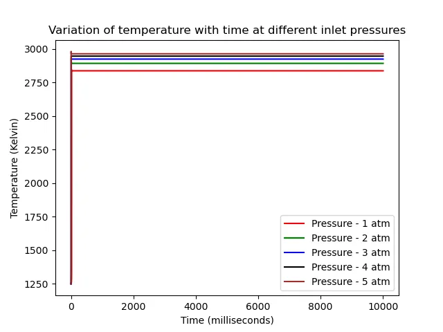
Inferences:

• It can be clearly seen that as pressure increases, the ignition delay is decreasing. This is because at high pressure, the latent heat of vapourization of the fuel would be low. Because of which the fuel molecules vapourize faster and so the ignition delay time decreases
• At the pressure five times the atmospheric pressure, the ignition dealy is so low that it is not visible even with the milli second scale. The temperature profile is almost linear, which implies instant combustion. So for a better combustion process and to reduce ignition delay time, high pressure is desired

B. Ignition delay time:

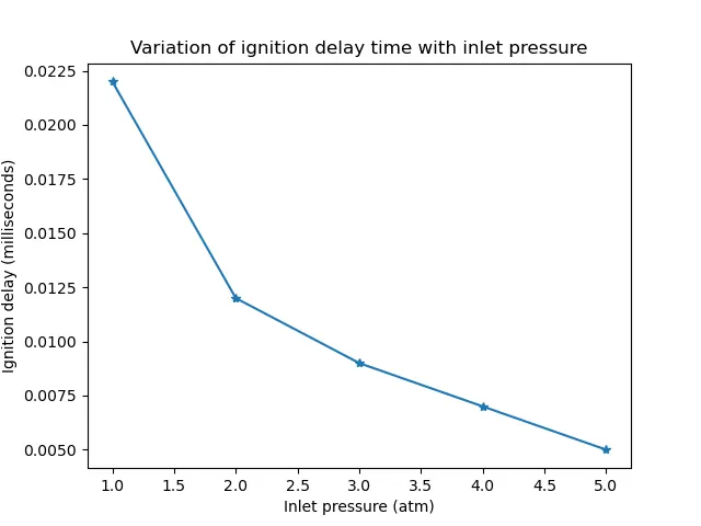
Effect of inlet pressure on ignition delay is,

Inferences:

• The ignition delay is significantly decreasing as inlet pressure increases. This is because of the reason mentioned above, which is, at high pressures the latent heat of vapourization of fuel will be less. So, the ignition process starts in relatively less time
• The decrement in ignition delay time value is relatively large between 1 atm and 2 atm and then remained almost constant till 5 atm. Increasing inlet pressure will lead to a quicker combustion

2. Effect of inlet temperature on ignition delay time:

For this simulation, the inlet pressure is kept constant at 5 atm and the temperature is varied from 950 K to 1450 K. The python code to execute this simulation is,

import sys
import numpy as np
import cantera as ct
import matplotlib.pyplot as plt

gas = ct.Solution('gri30.xml')
Temp = np.linspace(950,1450,5)
total_time = 10*1000
T_Auto = []
ignition_delay = []
P = 5*101325

for i in range(0,5):
	gas.TPX = Temp[i], P, {'CH4':1, 'O2':2, 'N2':7.52}
	r = ct.IdealGasReactor(gas)
	#help(r)
	sim = ct.ReactorNet([r])
	time = 0
	states = ct.SolutionArray(gas,extra=['time_in_milli_seconds','t'])
	temp_prev = Temp[i]

	for j in range (0,10000+1):
		time = time + 1e-3 
		sim.advance(time)
		states.append(r.thermo.state, time_in_milli_seconds = time*1e3, t = time)
		temp_new = states.T

		if (temp_new[j] - temp_prev) >= 400:
			ignition_delay.append(time)
		
		lee = states.T
		temp_prev = lee[j]


	if i == 0:
		temp_1 = states.T
	if i == 1:
		temp_2 = states.T
	if i == 2:
		temp_3 = states.T
	if i == 3:
		temp_4 = states.T
	if i == 4:
		temp_5 = states.T 


plt.figure(1)
plt.plot(states.time_in_milli_seconds,temp_1,color='red')
plt.plot(states.time_in_milli_seconds,temp_2,color='green')
plt.plot(states.time_in_milli_seconds,temp_3,color='blue')
plt.plot(states.time_in_milli_seconds,temp_4,color='black')
plt.plot(states.time_in_milli_seconds,temp_5,color='brown')

plt.legend(['Temperature - 950 K','Temperature - 1075 K','Temperature - 1200','Temperature - 1325 K','Temperature - 1450 K'])
plt.xlabel('Time (milliseconds)')
plt.ylabel('Temperature (Kelvin)')
plt.title('Variation of temperature in the reactor at different inlet temperatures')


plt.figure(2)
plt.plot(Temp,ignition_delay,'-*')
plt.xlabel('Inlet temperature (K)')
plt.ylabel('Ignition delay (milliseconds)')
plt.title('Variation of ignition delay time with inlet pressure')

plt.show()

When the above code is executed, the resultant plots are,

Results:

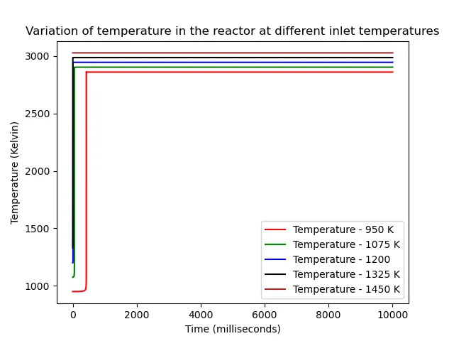
A. Temperature profiles throughout the combusiton at different inlet temperature values:

Inferences:

• Ignition delay time is clearly decreasing as the inlet temperature increases. As at high inlet temperatures, kinetic energy of the molecules (temperature) would be high and so less energy is reequired to vaporize them, so less time is required to ignite
• Ignition delay when the inlet temperature is 1450 K is very small that the temperature profile is almost flat, which imples instant ignition

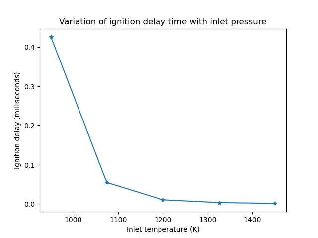
B. Effect of inlet temperature on ignition delay:

Inferences:

• Clearly ignition delay time is decreasing with increasing inlet temperature, for the reasons mentioned above
• Also, the rate of decrement of ignition delay time is more with increasing inlet temperature than with increasing inlet pressure. So to decrease the iginition delay time, increasing inlet temperature would give better results than increasing inlet pressure

3. Variation of molar concentrations of `H_2O, O_2 and OH` with time:

Python code to study the variation of molar concentrations of `H_2O, O_2 and OH` with time is,

import sys
import cantera as ct
import matplotlib.pyplot as plt
import numpy as np

gas = ct.Solution('gri30.xml')
Temp = np.linspace(500,1000,2) #K
P = 5*101325 #atm/bar

H2O_500 = []
O2_500 = []
OH_500 = []

H2O_1000 = []
O2_1000 = []
OH_1000 = []
	
for i in range(0,2):
	gas.TPX = Temp[i], P, {'CH4':1, 'O2':2, 'N2':7.52}
	r = ct.IdealGasReactor(gas)
	sim = ct.ReactorNet([r])
	time = 0
	states = ct.SolutionArray(gas,extra=['time_in_milli_seconds','t'])
	Temp_prev = Temp[i]

	for j in range(0,10000+1):
		time = time + 1e-3
		sim.advance(time)
		states.append(r.thermo.state,time_in_milli_seconds = time*1e3, t = time)
		Temp_new = states.T

		if i == 0:
			H2O_500 = (states.X[:,gas.species_index('H2O')])
			O2_500 = (states.X[:,gas.species_index('O2')])
			OH_500 = (states.X[:,gas.species_index('OH')])
		if i == 1:
			H2O_1000 = (states.X[:,gas.species_index('H2O')])
			O2_1000 = (states.X[:,gas.species_index('O2')])
			OH_1000 = (states.X[:,gas.species_index('OH')])

plt.figure(1)
plt.plot(states.t,H2O_500,color='red')
plt.xlabel('Time (sec)')
plt.ylabel('Molar concentration of H2O')
#plt.title('Variation of molar concentration of H2O with time at inlet temperature - 500 K')

plt.figure(2)
plt.plot(states.t,O2_500,color='blue')
plt.xlabel('Time (sec)')
plt.ylabel('Molar concentration of O2')
#plt.title('Variation of molar concentration of O2 with time at inlet temperature - 500 K')

plt.figure(3)
plt.plot(states.t,OH_500,color='green')
plt.xlabel('Time (sec)')
plt.ylabel('Molar concentration of OH')
#plt.title('Variation of molar concentration of OH with time at inlet temperature - 500 K')

plt.figure(4)
plt.plot(states.t,H2O_1000,color='red')
plt.xlabel('Time (sec)')
plt.ylabel('Molar concentration of H2O')
#plt.title('Variation of molar concentration of H2O with time at inlet temperature - 1000 K')

plt.figure(5)
plt.plot(states.t,O2_1000,color='blue')
plt.xlabel('Time (sec)')
plt.ylabel('Molar concentration of O2')
#plt.title('Variation of molar concentration of O2 with time at inlet temperature - 1000 K')

plt.figure(6)
plt.plot(states.t,OH_1000,color='green')
plt.xlabel('Time (sec)')
plt.ylabel('Molar concentration of OH')
#plt.title('Variation of molar concentration of OH with time at inlet temperature - 1000 K')

plt.show()

When the above code is executed the resultant plots are,

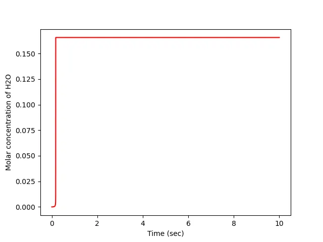
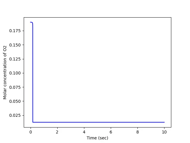
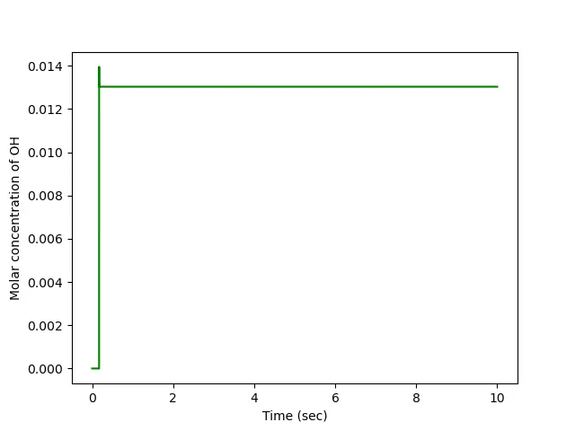
A. At inlet temperature - 1000 K and pressure - 5 bar:

`H_2O`:

Inferences:

• The time rate of change of molar concentration of `H_2O` is similar to a time rate of change of temperature. The water vapour in the air gets seperated and forms a product of the reaction. As the reaction progresses, the concentration of products increases and so, right after crossing the ignition delay time, the concentration of `H_2O` also increases instantly

`O_2`:

Inferences:

• Oxygen in the air is used by the fuel to combust and so right after passing the ignition delay time, ignition starts, which is a chemical reaction, which suddenly uses all the oxygen. So, the profile of `O_2` has a sudden fall at the same time where `H_2O` profile has a sudden rise

`OH`:

Inferences:

• OH is also a product of reaction and as the reaction progresses, its concentration increases. It can be safely concluded that time rate of change of concentration of products changes in a same way temperature varies as reaction progresses

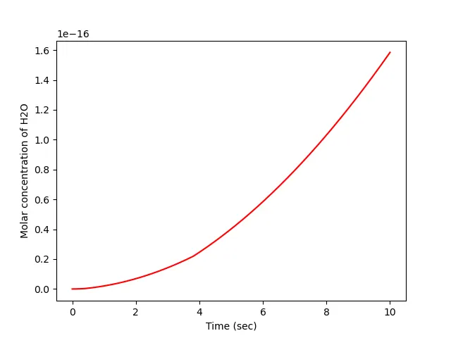
B. At inlet temperature - 500 K and pressure - 5 bar:

`H_2O`:

Inferences:

• As temperture is 500 K which is less than the auto ignition temperature or minimum temperature required for methane to get ignited, which is 873 K. So there isn't any chemical reaction taking place. The time rate of change of `H_2O` is because of the high pressure, which is 5 times the atmosphere, which is increasing the temperature (Gay Lussac's law), which is heating up the air and increasing the concentration of `H_2O` (water vapour)

`O_2`:

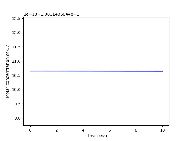
Inferences:

• As no reaction is taking place, the molar concentration of `O_2` is constant through out the time

OH:

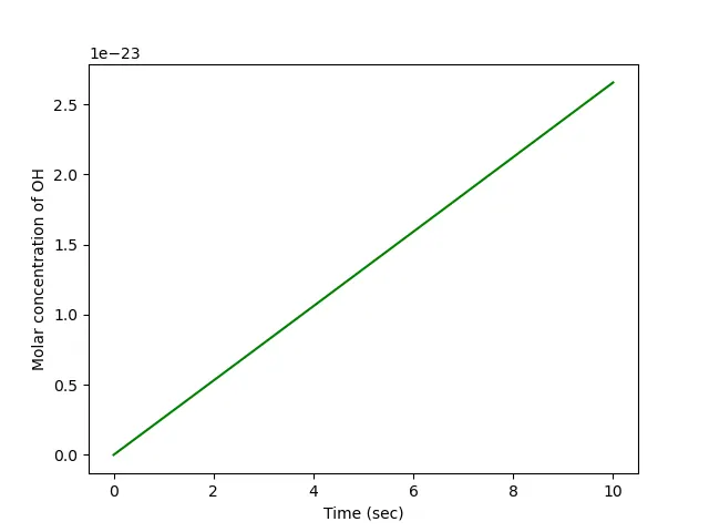
Inferences:

• The positive time rate of change of molar concentration of OH is because of the inlet pressure, which increases the temperature

Conclusions:

1. The effect of inlet pressure on auto ignition and ignition delay is plotted and studied. It can be concluded that ignition delay time decreases as the inlet pressure increases
2. The effect of inlet temperature on auto ignition and ignition delay is plotted and studied. The increase in inlet temperature has a decreasing effect on ignition delay time
3. The profile of time rate of change of products has a profile analogous to that of temperature, increasing tendency and the profile of time rate of change of species in reactants side has a decreasing tendency. When the temperature is 500K, the reaction did not take place and the time rate of change of oxygen was a horizontal line, which implies that the oxygen in the air has not been used