Week 7 - Auto ignition using Cantera
AIM:-
CASE I
To simulate the auto-ignition for methane for about 10 sec with 2 different condition
1. constant temperature of 1250K and pressure varying from 1 to 5 atm and plot the variation of autoignition time.
2.constant pressure of 5 atm and temperature varying from 950K to 1450K and plot the variation of autoignition time.
CASE II
Observe the rate of change of molar concentration under two conditions of the given elements "H2O, O2, OH" with respect to the time, (simulation time = 10 secs) under two different conditions
1.When Temperature is 1000K and pressure 5 bar.
2.When Temperature is 500K and pressure 5 bar.
THEORY:
The phenomena of autoignition when the mixture ignites spontaneously at a temperature called autoignition temperature kindling point of a substance is the lowest temperature in which it spontaneously ignites in a normal atmosphere without an external source of ignition, such as a flame or spark. The autoignition temperature is not an intrinsic property of the gases or vapours (Kanury 1975) but is the lowest temperature in a system where the rate of heat evolved from the gases or vapours increases beyond the rate of heat loss to the surroundings, resulting in the ignition. The autoignition temperature of a mixture of gases or vapours is affected by pressure, vessel shape and volume, surface activity, contaminants, flow rate, reaction rate, droplet and mist formation, gravity, and reactant concentration.
To compute the ignition time and ignition we assume a stoichiometric equation of methane using Cantera. Cantera uses Cantera Reactor that represents the simplest form of a chemically reacting system that is defining the governing equation. It corresponds to an extensive thermodynamic control volume V">V, in which all state variables are homogeneously distributed. The system is generally unsteady, i.e. all states are functions of time.In particular, transient state changes due to chemical reactions are possible. However, thermodynamic (but not chemical) equilibrium is assumed to be present throughout the reactor at all instants of time. In addition to single reactors, Cantera is also able to interconnect reactors into a Reactor Network, therefore, allowing the time integration. The use of time integrations thus make makes mandatory usage of reactor network even if one single reactor is being considered.
For this problem, we are defining an ideal gas reactor whose state variables are
m|kg| the mass of the reactant constant
V[`m^3`|the reactor volume
T|k|:The temperature
`Y_k`: The mass fraction for each species
The governing equation for reactor models are
Mass conservation
`(dm)/(dt)=sum_(i n)(\dot m)i n−sum_(out)(\dot m)out+(\dot m)wall`
Species conservation
The rate of change in the mass of each species is:
`(\dot m)_k,g en=V(\dot m)_kW_k+(\dot m)_(w a ll)`
`(d(mYk))/dt=sum_(i n){\dot {m}}_(i n)Y_k,(i n)−sum_(out){\dot {m}}_(out)Y_k+{\dot {m}}_(k,g en)`
Energy Conservation
`U=msum_(k)Y_ku_k(T)`
`(dU)/dt=u(dm)/dt+mc_v(dT)/dt+msum_(k)u_k(dY_k)/dt`
In this challenge, we will be solving the equation to determine the rate of change of temperature from where we could compute ignition delay
Step to solve Reactor Network
-
Define
Solutionobjects for the fluids to be flowing through your reactor network. -
Define the reactor type(s) and reservoir(s) that describe your system. Chose Ideal Gas (Constant Pressure) Reactor(s) if you only consider ideal gas phases.
-
Optional: Set up the boundary conditions and flow devices between reactors or reservoirs.
-
Define a reactor network which contains all the reactors previously created.
-
Advance the simulation in time, typically in a for- or while-loop. Note that only the current state is stored in Cantera by default. If you want to observe the transient states, you manually have to keep track of them.
-
Analyze the data.
CASE I
Autoignition time of methane with a constant temperature of 1250k and pressure varying the from 1 bar to 5bar.
import cantera as ct
import numpy as np
import matplotlib.pyplot as plt
import sys


gas=ct.Solution('gri30.xml')

#Defining the variables
Pressure = np.linspace(1,5,9)
T_ini=1250

#time of simulation is 10sec and in milli seconds 10000 that is taken as time step
n=10000

ignition_delay=[]
Temp_pres=[]
for P in Pressure:
	gas.TPX=T_ini,P*101325,{'CH4':1,'O2':2,'N2':7.52}

	Temp_autoignition=0
	time_autoignition=0
	time=0

	r=ct.IdealGasReactor(gas)
	sim=ct.ReactorNet([r])
	states=ct.SolutionArray(gas,extra=['time_in_ms','t'])
	print('{:10s} {:10s} {:10s}'.format('t[s]','T[K]','P[Pa]'))


	for n in range(n):

		time+=1e-3
		sim.advance(time)
		states.append(r.thermo.state,time_in_ms=time*1e3,t=time)
		print('{:10.2e} {:10.2f} {:10.2f}'.format(sim.time,r.T,r.thermo.P))


	Temp_pres.append(states.T)


	for i in range(n):
		T_error = states.T[i] - T_ini - 400
		if T_error > 0:
			Temp_autoignition = states.T[i]
			time_autoignition = states.time_in_ms[i]
			break

	ignition_delay.append(time_autoignition)

Temp_pres=np.array(Temp_pres)
#plot for Variation of Autoigniton Temperature with variation in inlet different inlet pressure and at an inlet temperature  of 1250[K]
for k in range(len(Pressure)):
	plt.plot(Temp_pres[k])
	plt.title('Variation of Autoigniton Temperature with\n   different inlet pressure and constant inlet temperature  of 1250[K]')
	plt.xlabel('Number of time steps',fontsize=12)
	plt.ylabel('Temperature',fontsize=12)
	plt.legend(['1 atm', '1.5 atm', '2 atm', '2.5 atm', '3 atm', '3.5 atm', '4 atm', '4.5 atm', '5 atm'])
plt.show()

# Plot for Ignition delay vs Pressure
plt.figure (2)
plt.plot(Pressure,ignition_delay,'-o')
plt.title(('Ignition delay vs Pressure'))
plt.xlabel('Pressure',fontsize=12)
plt.ylabel('Auto igniton Delay time [ms]',fontsize=12)
plt.show()
Results
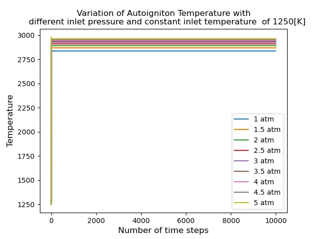
Figure.1
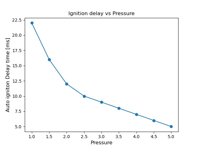
Figure.2
PART II
Autoignition time of methane with a constant pressure of 5 bar and temperature varying the from 950 bar to 1450bar.
import cantera as ct
import numpy as np
import matplotlib.pyplot as plt
import sys


gas=ct.Solution('gri30.xml')


#Defining the variables
Temperature = np.linspace(950,1450,11)
P=5*101325
#time of simulation is 10sec and in milli seconds 10000 that is taken as time step
n=10000

#Array for storing ignition delay and and temperature at different tmperature
ignition_delay=[]
Temp_temp=[]

for T in Temperature:
	gas.TPX=T,P,{'CH4':1,'O2':2,'N2':7.52}

	Temp_autoignition=0
	time_autoignition=0
	time=0

	r=ct.IdealGasReactor(gas)
	sim=ct.ReactorNet([r])
	states=ct.SolutionArray(gas,extra=['time_in_ms','t'])
	print('{:10s} {:10s} {:10s}'.format('t[s]','T[K]','P[Pa]'))


	for n in range(n):

		time+=1e-3
		sim.advance(time)
		states.append(r.thermo.state,time_in_ms=time*1e3,t=time)
		print('{:10.2e} {:10.2f} {:10.2f}'.format(sim.time,r.T,r.thermo.P))


	Temp_temp.append(states.T)


	for i in range(n):
		T_error = states.T[i] - T - 400
		if T_error > 0:
			Temp_autoignition = states.T[i]
			time_autoignition = states.time_in_ms[i]
			break

	ignition_delay.append(time_autoignition)

Temp_temp=np.array(Temp_temp)

#plot for Variation of Autoigniton Temperature withvariation in inlet different inlet temperature at presure of 5bar
for k in range(len(Temperature)):
	plt.figure(1)
	plt.plot(Temp_temp[k])
	plt.title('Variation of Autoigniton Temperature with\n different inlet temperature and constant presure of 5bar')
	plt.xlabel('Number of time steps',fontsize=12)
	plt.ylabel('Temperature',fontsize=12)
	plt.legend(['950 k', '975k', '1000 k', '1025 k', '1050 k', '1075 k', '1100 k', '1125 k', '1150 k', '1175 k', '1200 k', '1225 k', '1250 k', '1275 k', '1300 k', '1325 k', '1350 k', '1375 k', '1400 k', '1425 k', '1450 k'])

#Plot Ignition delay vs Temperature
plt.figure (2)
plt.plot(Temperature,ignition_delay,'-o')
plt.title(('Ignition delay vs Temperature'))
plt.xlabel('Temperature [k]',fontsize=12)
plt.ylabel('Auto igniton Delay time [ms]',fontsize=12)
plt.show()
Results
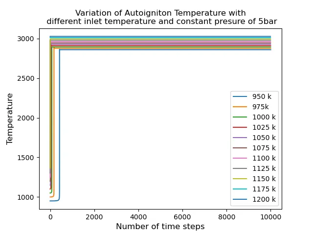
Figure.3
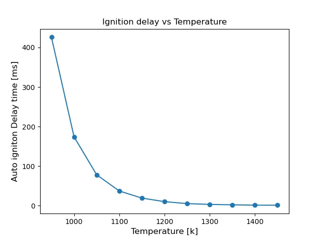
Figure.4
From both condition's graphs, it inferred that with the less value of pressure and temperature at the initial results in very large ignition delay that it took 400sec at a temperature of 950k and 1bar pressure to attain auto ignition and with increasing the condition the auto-ignition phenomena was quick and took nearly took 0 sec at the last condition's value.
CASE II
Observe the rate of change of molar concentration under two conditions of the given elements "H2O, O2, OH" with respect to the time, (simulation time = 10 secs) under two different conditions
1.When Temperature is 1000K and pressure 5 bar.
2.When Temperature is 500K and pressure 5 bar.
import cantera as ct
import numpy as np
import matplotlib.pyplot as plt
import sys

gas=ct.Solution('gri30.xml')

#Defining the variables
P=5*101325
#time of simulation is 10sec and in milli seconds 10000 that is taken as time step
n=10000

#Defining a function
def mole_fraction(T,P):
	gas.TPX=T,P,{'CH4':1,'O2':2,'N2':7.52}
	r=ct.IdealGasReactor(gas)
	sim=ct.ReactorNet([r])
	time=0
	states=ct.SolutionArray(gas,extra=['time_in_ms','t'])


	for i in range(n):

		time+=1e-3
		sim.advance(time)
		states.append(r.thermo.state,time_in_ms=time*1e3,t=time)

	return(states.T,states.t,states.X[:,gas.species_index('H2O')],states.X[:,gas.species_index('O2')],states.X[:,gas.species_index('OH')])


#Assinging theh value of function that is inital temperature of 500k and pressure of 5 bar

[Temp_mole,time_mole,ml_H20,ml_O2,ml_OH]	= mole_fraction(500,P)

#Plot  rate of change of molar concentration at temperature of 500k and pressure of 5 bar
plt.figure(1)

plt.subplot(3,1,1)
plt.title('Rate of Change of Molar Concentration at\n temperature of 500k and pressure of 5 bar')
plt.plot(time_mole,ml_H20,'b')
plt.xlabel('Time(sec)',fontsize=12)
plt.ylabel('H2O',fontsize=12)

plt.subplot(3,1,2)
plt.plot(time_mole,ml_O2,'r')
plt.xlabel('Time(sec)',fontsize=12)
plt.ylabel('O2',fontsize=12)

plt.subplot(3,1,3)
plt.plot(time_mole,ml_OH,'g')
plt.xlabel('Time(sec)',fontsize=12)
plt.ylabel('OH',fontsize=12)
plt.tight_layout()
plt.show()

#Assinging theh value of function that is inital temperature of 500k and pressure of 5 bar
[Temp_mole_1,time_mole_1,ml_1_H20,ml_1_O2,ml_1_OH]	= mole_fraction(1000,P)

#Plot  rate of change of molar concentration at temperature of 1000k and pressure of 5 bar
plt.figure(2)
plt.subplot(3,1,1)
plt.title('Rate of Change of Molar Concentration at\ntemperature of 1000k and pressure of 5 bar')
plt.plot(time_mole_1,ml_1_H20,'b')
plt.xlabel('Time(sec)',fontsize=12)
plt.ylabel('H2O',fontsize=12)

plt.subplot(3,1,2)
plt.plot(time_mole_1,ml_1_O2,'r')
plt.xlabel('Time(sec)',fontsize=12)
plt.ylabel('O2',fontsize=12)

plt.subplot(3,1,3)
plt.plot(time_mole_1,ml_1_OH,'g')
plt.xlabel('Time(sec)',fontsize=12)
plt.ylabel('OH',fontsize=12)
plt.tight_layout()
plt.show()

# Plot for Auto igniton Temperature Variation at two different intial temperature of 1000 K and 500K with constant pressure of 5bar
plt.figure(3)
plt.title("Auto igniton Temperature Variation at\n two different intial temperature of 1000 K and 500K with constant pressure of 5bar")
plt.plot(time_mole_1,Temp_mole_1,label='1000 K')
plt.plot(time_mole,Temp_mole,label='500 K')
plt.xlabel("Time(sec)",fontsize=12)
plt.ylabel("temperature [K]",fontsize=12)
plt.show()
Results
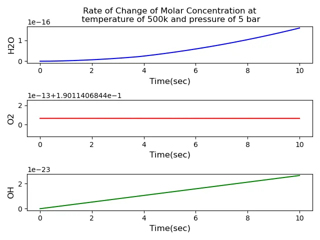
Figure.5
Here the with a low initial temperature of 500k, the auto-ignition is very slow. The O2 shows no variation in its molar concentration and remained constant throughout the 10 sec period this prooves that no occurrence of combustion. The concentration of the products OH and H20 are nearly negligible are. Therefore it can be concluded that with low initial temperature the auto-ignition doest take place
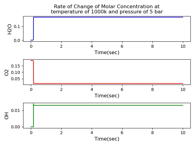
Figure.6
The 1000k initial temperature shows that autoignition occurred with a lesser amount of ignition delay. in addition, it showed that increase in mole fraction OH and H20 while also displayed a drop in O2, it is because O2 reacts with fuel for combustion. The pattern for the change in mole fraction all 3 species is identical and consistent.
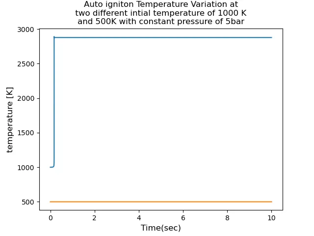
Figure.7
The reasons above mentioned and their conclusion can be seen this plot