Week 6 - Multivariate Newton Rhapson Solver
Given Data
`(dy_1)/dt=-0.04y_1+10^4y_2y_3`
`(dy_2)/dt=0.04y_1-10^4y_2y_3-3*10^7y_2^2`
`(dy_3)/dt=3*10^7*y_2^2`
alpha=1
time(t)=10 min
initial guess value
y1=1
y2=0
y3=0
To Find
Solve the problem using Implicit Euler Method/Backward Differencing
suitable step size, reason for choosing that step size
Solution
solve y variable f(t)
General
`y_(New)=y_(old)-alpha*(J^-1*F)`
matrix form
`[[Y_(New1)],[Y_(New2)],[Y_(New3)]]=[[Y_(old1)],[Y_(old2)],[Y_(old3)]]-alpha*[[(df_1)/(dy_1 )(df_1)/(dy_2 )(df_1)/(dy_3 )],[(df_2)/(dy_1 )(df_2)/(dy_2 )(df_2)/(dy_3 )],[(df_3)/(dy_1 )(df_3)/(dy_2 )(df_3)/(dy_3 )]]*[[f1],[f2],[f3]]`
Converting differential form to programming to calculate the given condition
ODE
`(dy_1)^(n-1)=(-0.04y_1^(n)+10^4y_2^(n)y_3^(n))*dt+dy_1^(n)`
`(dy_2)^(n-1)=(0.04y_1-10^4y_2y_3-3*10^7y_2^2)*dt+dy_2^(n)`
`(dy_3)^(n-1)=(3*10^7*y_2^2)*dt+(dy_3)^(n)`
`f_1=(dy_1)^(n-1)-(0.04y_1(n)+10^4y_2(n)y_3(n))*dt-dy_1(n)=0`
`f_2=(dy_2)^(n-1)+(0.04y_1-10^4y_2y_3-3*10^7y_2^2)*dt-dy_2^(n)=0`
`f_3=dy_3^(n-1)+(3*10^7*y_2^2)*dt-dy_3^(n)=0`
simply converting jacobian
`[[(f_(New1)-f_(old1))/(dy_1 )(f_(New1)-f_(old1))/(dy_2 )(f_(New1)-f_(old1))/(dy_3 )],[(f_(New2)-f_(old2))/(dy_1 )(f_(New2)-f_(old2))/(dy_2 )(f_(New2)-f_(old2))/(dy_3 )],[(f_(New3)-f_(old3))/(dy_1 )(f_(New3)-f_(old3))/(dy_2 )(f_(New3)-f_(old3))/(dy_3 )]]`
creating a dummy solution value to store old value, apply constrain and Framing Newton Raption method
Euler’s method is a numerical method to solve first order first-degree differential equation with a given initial value. It is the most basic explicit method for numerical integration of ordinary differential equations
Newton Rapson Method
the solution starts from initial guess variables of variable
from rewrite function `f(y)` using a Taylor series expansion in `(y_(New)-y_(old))`:
`f(y)=f(y_0)+f'(y_0)f(y-y_0)+1/2*f''(y_0)(y-y_0)^2+...=0`
from accounting to derivative that `y_i` can be written as
`y_i=y_i-f(y_i)/(f'(y_i))`
below are reference for nodel solution
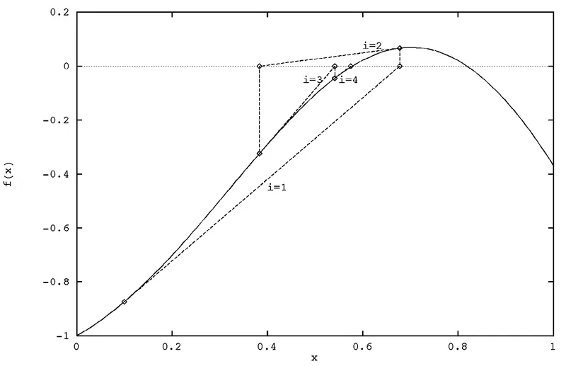
N-R method finds the tangent to the function `f(t)` at y=y0 and extrapolates it to intersect the x-axis to get t1. This point of intersection is taken as the new approximation to the root and the procedure is repeated until convergence is obtained whenever possible. given the value of y = yi at the end of the ith iteration till the solution converge
creating a function to define implicitly method inside a time loop
Given input guess value for variable and time constraint to solve the equation
Python code
"""
#Given
#dy1/dt=-0.04y1+10^4y2y3
#dy2/dt=0.04y1-10^4y2y3-3*10^7y2^2
#dy3/dt=3*10^7*y2^2

derivative form
#dy1(n-1)=(-0.04y1(n)+10^4y2(n)y3(n)))*dt+dy1(n)
#dy2(n-1)=(0.04y1-10^4y2y3-3*10^7y2^2)*dt+dy2(n)
#dy3(n-1)=(3*10^7*y2^2)*dt+dy3(n)

BDF using multivariate newtonRapson method f=dyvariant(n+1)-dyvariant(n)=0 so rewrite
#f1=dy1(n-1)+((-0.04y1(n)+10^4y2(n)y3(n)))*dt-dy1(n))=0
#f2=dy2(n-1)+((0.04y1-10^4y2y3-3*10^7y2^2)*dt-dy2(n))=0
#f3=dy3(n-1)+((3*10^7*y2^2)*dt-dy3(n))=0

"""

import math
import matplotlib.pyplot as plt
import numpy as np
from numpy.linalg import inv

a=0.04
b=pow(10,4)
c=3*pow(10,7)

def S1(y1,y2,y3,y1_new,y2_new,y3_new,h):
	return y1+h*((-a*y1_new)+(b*y2_new*y3_new))-y1_new
def S2(y1,y2,y3,y1_new,y2_new,y3_new,h):
	return y2+h*((a*y1_new)-(b*y2_new*y3_new)-(c*(y2_new**2)))-y2_new
def S3(y1,y2,y3,y1_new,y2_new,y3_new,h):
	return y3+h*(c*(y2_new**2))-y3_new

def jacobian(y1,y2,y3,y1_new,y2_new,y3_new,h):
	#jacobian
	J=np.ones((3,3))
	dy=1e-9


	J[0,0]=(S1(y1,y2,y3,(y1_new+dy),y2_new,y3_new,h)-S1(y1,y2,y3,y1_new,y2_new,y3_new,h))/dy
	J[0,1]=(S1(y1,y2,y3,y1_new,(y2_new+dy),y3_new,h)-S1(y1,y2,y3,y1_new,y2_new,y3_new,h))/dy
	J[0,2]=(S1(y1,y2,y3,y1_new,y2_new,(y3_new+dy),h)-S1(y1,y2,y3,y1_new,y2_new,y3_new,h))/dy

	J[1,0]=(S2(y1,y2,y3,(y1_new+dy),y2_new,y3_new,h)-S2(y1,y2,y3,y1_new,y2_new,y3_new,h))/dy
	J[1,1]=(S2(y1,y2,y3,y1_new,(y2_new+dy),y3_new,h)-S2(y1,y2,y3,y1_new,y2_new,y3_new,h))/dy
	J[1,2]=(S2(y1,y2,y3,y1_new,y2_new,(y3_new+dy),h)-S2(y1,y2,y3,y1_new,y2_new,y3_new,h))/dy

	J[2,0]=(S3(y1,y2,y3,(y1_new+dy),y2_new,y3_new,h)-S3(y1,y2,y3,y1_new,y2_new,y3_new,h))/dy
	J[2,1]=(S3(y1,y2,y3,y1_new,(y2_new+dy),y3_new,h)-S3(y1,y2,y3,y1_new,y2_new,y3_new,h))/dy
	J[2,2]=(S3(y1,y2,y3,y1_new,y2_new,(y3_new+dy),h)-S3(y1,y2,y3,y1_new,y2_new,y3_new,h))/dy

	return J
# Newton Rapson
def NR(y1,y2,y3,y1_guess,y2_guess,y3_guess,h):

	s_old=np.ones((3,1))
	s_old[0]=y1_guess
	s_old[1]=y2_guess
	s_old[2]=y3_guess

	F=np.ones((3,1))

	# constraining criteria
	error=9e9
	tol=1e-9
	alpha=1

	iter=1

	while error > tol:
		J=jacobian(y1,y2,y3,s_old[0],s_old[1],s_old[2],h)

		F[0]=S1(y1,y2,y3,s_old[0],s_old[1],s_old[2],h)
		F[1]=S2(y1,y2,y3,s_old[0],s_old[1],s_old[2],h)
		F[2]=S3(y1,y2,y3,s_old[0],s_old[1],s_old[2],h)

		s_new=s_old-alpha*(np.matmul(inv(J),F))

		error=np.max(np.abs(s_new-s_old))

		s_old=s_new

		iter=iter+1

	return[s_new[0],s_new[1],s_new[2]]

def implicit_euler(iny1,iny2,iny3,tsp,dt):

	t=np.arange(0,tsp,dt)
	y1=np.zeros(len(t))
	y2=np.zeros(len(t))
	y3=np.zeros(len(t))

	y1[0]=iny1
	y2[0]=iny2
	y3[0]=iny3

	y1_guess=0
	y2_guess=1
	y3_guess=1

	for i in range(1,len(t)):

		y1[i],y2[i],y3[i]=NR(y1[i-1],y2[i-1],y3[i-1],y1_guess,y2_guess,y3_guess,dt)

		y1_guess=y1[i]
		y2_guess=y2[i]
		y3_guess=y3[i]


	return[t,y1,y2,y3]

tint=0
tfin=10*60
#Number of points
nps=[3,6,30,60,300,500]
dt=np.arange(0,tfin,nps[5])
print('number of points=',np.size(dt))
# input values for implicit euler
t,y1,y2,y3=implicit_euler(1,0,0,600,dt[1])

plt.plot(t,y1,'b')
plt.plot(t,y2,'m')
plt.plot(t,y3,'r')
plt.title('Y variable vs time ')
plt.xlabel('time')
plt.ylabel('y1 y2 y3')
plt.legend(["y1","y2","y3"])
plt.grid(color='orange',linestyle='--',linewidth=0.6)
plt.show()
Graph
Time Vs Y variables
dt=3 number of points in between 200
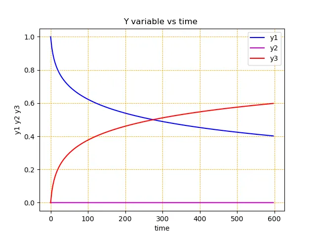
dt=6 number of points in between 100
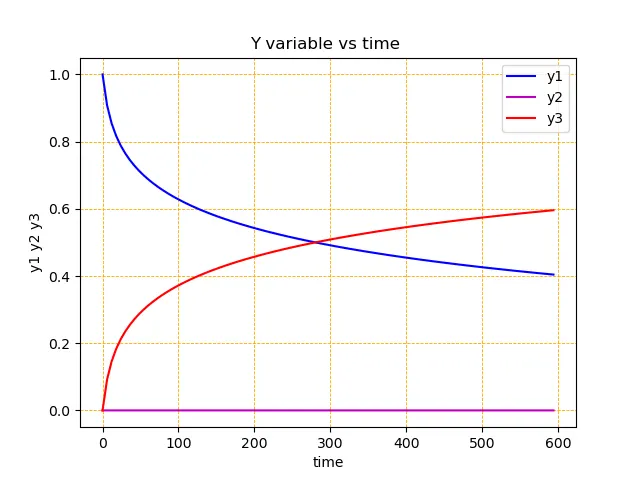
dt=30 number of points in between 20
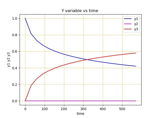
dt=60 number of points in between 10
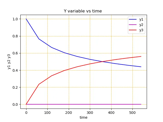
dt=300 number of points in between 2
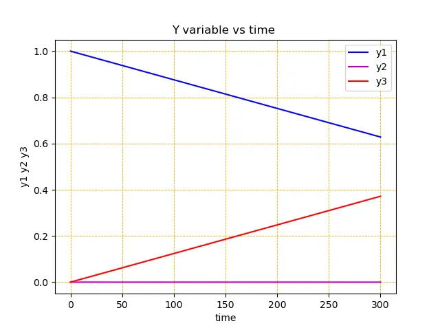
validate Result at different time step
| S.No | Time Step | Nodes | Solution selection |
| 1 | 3 | 200 | smooth good result |
| 2 | 6 | 100 | smooth good & time-saving result(best) |
| 3 | 30 | 20 | ok to check the result but more time step to get a smooth curve |
| 4 | 60 | 10 | ok to check the solution in the right direction |
| 5 | 300 | 2 | worst need more time-step to get an accurate result |
Result
Implicit Euler is numerical stable for all time step but lesser time step gives smoothness of result
Better to choose time step (dt)=6 for faster calculation and smooth output of the result
References
https://web.mit.edu/10.001/Web/Course_Notes/NLAE/node6.html
https://www.kth.se/social/files/54187f60f276542277f51f08/lec05.pdf
skill Lync Team