Week 6 - Multivariate Newton Rhapson Solver

Aim:-

To find the solution for non-linear ordinary differential equations using Newton Raphsom's method, incorporating or including an implicit(Euler's backward differencing) scheme.

ODE system:

`dy_1/dt = -0.04y_1 + 10^4y_2y_3`

`dy_2/dt = 0.04y_1 - 10^4y_2y_3- 3*10^7y_2^2`

`dy_3/dt = 3*10^7y_2^2`

The basic formula for implicit method:

`y_i^n = y_1^(n-1) + h*((dy)/(dt))^n`

The ODE system was converted into above form:

`y_1^n = y_1^(n-1) + h*(-0.04*y_1 + 10^4*y_2*y_3)`

`y_2^n = y_2^(n-1) + h*(0.04*y_1-10^4*y_2*y_3-3*10^7*y_2^2)`

`y_3^n = y_3^(n-1) + h*(3*10^7*y_2^2)`

or converting the above equations to non-linear equations by bringing LHS to RHS. RHS - LHS = 0.

`f_1 =y_1^(n-1) + h*(-0.04*y_1 + 10^4*y_2*y_3)-y_1^n = 0`

`f_2=y_2^(n-1) + h*(0.04*y_1-10^4*y_2*y_3-3*10^7*y_2^2) - y_2^n= 0`

`f_3=y_3^(n-1) + h*(3*10^7*y_2^2) - y_3^n = 0`

F is the column vector:

F = `((f_1),(f_2),(f_3))`

Newton Raphsom's method:-

It is a root-finding algorithm that produces successively better approximations to the roots(or zeroes) of a real-valued function. Here, an implicit differential scheme is using because the system is a stiff system. The equation for Newton Raphsom's method is mentioned below:

`Y_(n+1) = Y_(old) + alpha*J^(-1)*F`

Ynew = `Y_(n+1)` = New value updated after every iteration.

Yguess = `y_(old)`

`alpha` = Relaxation factor = 1

J = Jacobian matrix

F = Function matrix

J = `[((delf_1)/(dely_1),(delf_1)/(dely_2),(delf_1)/(dely_3)),((delf_2)/(dely_1),(delf_2)/(dely_2),(delf_2)/(dely_3)),((delf_3)/(dely_1),(delf_3)/(dely_2),(delf_3)/(dely_3))]`

By substituting all in Newton Raphsom's method, we get:

`[(y_1^text(new)),(y_2^text(new)),(y_3^text(new))]=[(y_(1old)),(y_(2old)),(y_(3old))]-alpha*[((delf_1)/(dely_1),(delf_1)/(dely_2),(delf_1)/(dely_3)),((delf_2)/(dely_1),(delf_2)/(dely_2),(delf_2)/(dely_3)),((delf_3)/(dely_1),(delf_3)/(dely_2),(delf_3)/(dely_3))]^-1* [(f_1),(f_2),(f_3)]`

Code:-

"""
Solving a set of ODE using multivariate newton raphson method
	dy1/dt = -0.04*y1 + 10^4*y2*y3 - 3*10^7*y2^2
	dy2/dt = 0.04*y1 - 10^4*y2*y3 - 3*10^7*y2^2
	dy3/dt = 3*10^7*y2^2
"""

import numpy as np
import matplotlib.pyplot as plt
from numpy.linalg import inv

def f1(y1_o,y1,y2,y3,dt):
	return (y1_o + dt*(-0.04*y1 + pow(10,4)*y2*y3) - y1)

def f2(y1,y2_o,y2,y3,dt):
	return (y2_o + dt*(0.04*y1 - pow(10,4)*y2*y3 - 3*pow(10,7)*pow(y2,2)) - y2)

def f3(y1,y2,y3_o,y3,dt):
	return (y3_o + dt*(3*pow(10,7)*pow(y2,2)) - y3)

def J(y1_o,y1,y2_o,y2,y3_o,y3,dt):

	dy = 1e-4
	J = np.ones((3,3))

	# Defining the first row of jacobian matrix
	J[0,0] = (f1(y1_o,y1+dy,y2,y3,dt) - f1(y1_o,y1,y2,y3,dt))/dy
	J[0,1] = (f1(y1_o,y1,y2+dy,y3,dt) - f1(y1_o,y1,y2,y3,dt))/dy
	J[0,2] = (f1(y1_o,y1,y2,y3+dy,dt) - f1(y1_o,y1,y2,y3,dt))/dy

	# Defining the second row of jacobian matrix
	J[1,0] = (f2(y1+dy,y2_o,y2,y3,dt) - f2(y1,y2_o,y2,y3,dt))/dy
	J[1,1] = (f2(y1,y2_o,y2+dy,y3,dt) - f2(y1,y2_o,y2,y3,dt))/dy
	J[1,2] = (f2(y1,y2_o,y2,y3+dy,dt) - f2(y1,y2_o,y2,y3,dt))/dy

	# Defining the third row of jacobian matrix
	J[2,0] = (f3(y1+dy,y2,y3_o,y3,dt) - f3(y1,y2,y3_o,y3,dt))/dy
	J[2,1] = (f3(y1,y2+dy,y3_o,y3,dt) - f3(y1,y2,y3_o,y3,dt))/dy
	J[2,2] = (f3(y1,y2,y3_o,y3+dy,dt) - f3(y1,y2,y3_o,y3,dt))/dy

	return J

#  Defining initial conditions

y1 = 1
y2 = 0
y3 = 0

# Defining the Y matrix

y_old = np.ones((3,1))

y_old[0] = y1
y_old[1] = y2
y_old[2] = y3

# Defining the F matrix

F = np.copy(y_old)
y_new = np.copy(y_old)

tol = 1e-4     # Defining the tolerance

alpha = 1    # Defining the relaxation factor

t_total = 600

dt = 0.1

L_1 = []
L_2 = []
L_3 = []
iter =1
repitation= []

a = np.arange(1,t_total,dt)

for i in range(0,len(a)):
	
	error = 9e9

	while(error > tol):

		F[0,0] = f1(y_old[0,0],y_new[0,0],y_new[1,0],y_new[2,0],dt)
		F[1,0] = f2(y_new[0,0],y_old[1,0],y_new[1,0],y_new[2,0],dt)
		F[2,0] = f3(y_new[0,0],y_new[1,0],y_old[2,0],y_new[2,0],dt)

		y_new = y_old - alpha*np.matmul(inv(J(y_old[0,0],y_new[0,0],y_old[1,0],y_new[1,0],y_old[2,0],y_new[2,0],dt)), F)

		error = max(abs(y_new-y_old))
		print(error)
			
		y_old = y_new
	
		log_message = 'repitation No. = {0} y1 = {1} y2 = {2} y3 = {3}'.format(iter,y_new[0],y_new[1],y_new[2])
		print(log_message)
		
		L_1.append(y_new[0])
		L_2.append(y_new[1])
		L_3.append(y_new[2])

		iter = iter+1
		repitation.append(iter)


fig1,ax1 = plt.subplots()
plt.plot(repitation,L_1,color = 'g')
plt.plot(repitation,L_2,color = 'm')
plt.plot(repitation,L_3,color = 'r')
plt.xlabel('Time (sec)')
plt.ylabel('Y')
plt.title('Variation of Y with time-dt = '+str(dt),fontsize=12,fontweight='bold')
plt.legend(['y1','y2','y3'],fontsize=10)
plt.show()

Plot:-

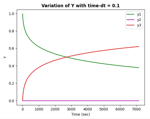
For dt = 0.1

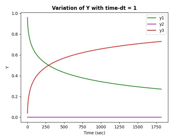
For dt = 1

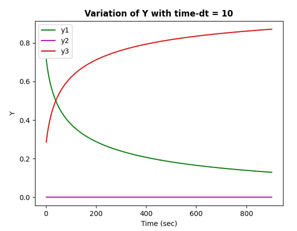
For dt = 10

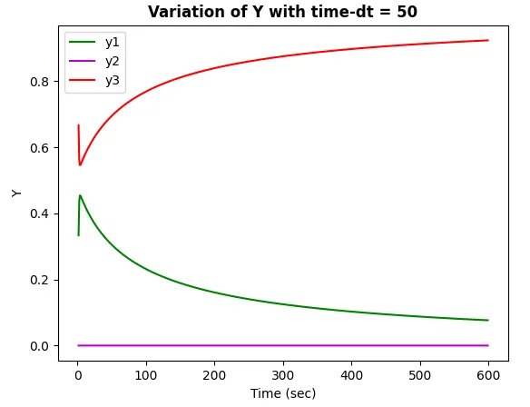
For dt = 50

Conclusion:-

An implicit function is not sensitive to step size but the accuracy of a system disturbs when we use the larger time step. As the value of the increases, the guess values seem to not align with initial guess values.