Week 6 - Multivariate Newton Rhapson Solver

INTRODUCTION

The combustion process is mostly governed by the chemical reactions that take place during the process. For simulating a combustion process, one of the most important things is calculating the concentration of the species produced during the process. The rate of generation or consumption of these chemical species is usually governed by a set of coupled stiff ordinary differential equations. In this study, we are using python to solve the coupled ODEs using the multivariate Newton Ralphson Method.

The ODEs that are solved in this study is shown below:

\begin{equation}
\frac{d y_{1}}{d t}=-0.04 y_{1}+10^{4} y_{2} y_{3}
\end{equation}

\begin{equation}
\frac{d y_{2}}{d t}=0.04 y_{1}-10^{4} y_{2} y_{3}-3 \cdot 10^{7} y_{2}^{2}
\end{equation}

\begin{equation}
\frac{d y_{3}}{d t}=3 \cdot 10^{7} y_{2}^{2}
\end{equation}

The equations that shown above rresembles the reaction rate equations where `y_1, y_2` and `y_3` represents the species involved in the reaction. By looking at the equations we know that the equations are coupled. These kind of equations can be solved using the multivariate Newton-Ralphson Technique. 

DERIVATION OF THE NUMERICAL SCHEME

The discretization is done using the Implicit Euler Method. The differential equations in the Implicit Euler scheme is shown below:

`\frac{y_{1}^{n+1}-y_{1}^{n}}{\Delta t}= -0.04y_{1}^{n+1} +10^{4}y_{2}^{n+1}y_{3}^{n+1}`

`\frac{y_{2}^{n+1}-y_{2}^{n}}{\Delta t}= 0.04y_{1}^{n+1} -10^{4}y_{2}^{n+1}y_{3}^{n+1}-3\times10^{7}(y_{2}^{n+1})^2`

`\frac{y_{3}^{n+1}-y_{3}^{n}}{\Delta t}=3\times10^{7}(y_2^{n+1})^2`

The superscripts `n` and `n+1` represents the previous and the current time step. Newton-Raphson methods are root finding problems so we can re write the above equations as shown below:

`f_1 = y_{1}^{n}+(-0.04y_{1}^{n+1}+10^{4}y_{2}^{n+1}y_{3}^{n+1})\Delta t -y_{1}^{n+1}=0`

`f_2 = y_{2}^{n}+(0.04y_{1}^{n+1}-10^{4}y_{2}^{n+1}y_{3}^{n+1}-3\times10^{7}(y_{2}^{n+1})^2)\Delta t -y_{2}^{n+1}=0`

`f_3 = y_{3}^{n}+(3\times10^{7}(y_{2}^{n+1})^2)\Delta t -y_{3}^{n+1}=0`

For continuous and differentiable functions `f(x)=0` the roots can be calculated using the formula `x_{n+1}= x_{n}-\frac{f(x)}{f\prime(x)}`

The equation can be modified using a relaxation factor as `x_{n+1}= x_{n}-\alpha \frac{f(x)}{f\prime(x)}`

For a multivariate equation the above equation can be written as `Y_{n+1} = Y_{n}-\alpha J^{-1}F`, where `Y` is the solution vector, `J` is the jacobian matrix and `F` is the function matrix.

`\begin{gather} J= \begin{bmatrix} \frac{\partial f_1}{\partial y_1} &\frac{\partial f_1}{\partial y_2}&\frac{\partial f_1}{\partial y_3}\\\frac{\partial f_2}{\partial y_1}&\frac{\partial f_2}{\partial y_2}&\frac{\partial f_2}{\partial y_3}\\\frac{\partial f_3}{\partial y_1}&\frac{\partial f_3}{\partial y_2}&\frac{\partial f_3}{\partial y_3} \end{bmatrix} \end{gather}`

`\begin{gather} F = \begin{bmatrix} f_1 \\ f_2\\f_3 \end{bmatrix} \end{gather}`

"""
Created on Wed Feb  3 22:27:03 2021

@author: jithu
"""

import numpy as np
import matplotlib.pyplot as plt
from numpy.linalg import inv


def f1(y1old,y1,y2,y3,h):
	return (y1old + h*(-0.04*y1 + y2*y3*1e4) - y1)

def f2(y2old,y1,y2,y3,h):
	return (y2old + h*(0.04*y1 - (1e4*y2*y3) -(3e7*y2*y2)) -y2)

def f3(y3old,y1,y2,y3,h):
	return (y3old + h*(3e7*y2*y2) - y3)

def jac(y1old,y2old,y3old,y1,y2,y3,h):


	J = np.ones((3,3))
	Δy = 1e-8    # Step size

	J[0,0] = (f1(y1old,y1+Δy,y2,y3,h)-f1(y1old,y1,y2,y3,h))/Δy 
	J[0,1] = (f1(y1old,y1,y2+Δy,y3,h)-f1(y1old,y1,y2,y3,h))/Δy 
	J[0,2] = (f1(y1old,y1,y2,y3+Δy,h)-f1(y1old,y1,y2,y3,h))/Δy 

	J[1,0] = (f2(y2old,y1+Δy,y2,y3,h)-f2(y2old,y1,y2,y3,h))/Δy 
	J[1,1] = (f2(y2old,y1,y2+Δy,y3,h)-f2(y2old,y1,y2,y3,h))/Δy 
	J[1,2] = (f2(y2old,y1,y2,y3+Δy,h)-f2(y2old,y1,y2,y3,h))/Δy

	J[2,0] = (f3(y3old,y1+Δy,y2,y3,h)-f3(y3old,y1,y2,y3,h))/Δy 
	J[2,1] = (f3(y3old,y1,y2+Δy,y3,h)-f3(y3old,y1,y2,y3,h))/Δy
	J[2,2] = (f3(y3old,y1,y2,y3+Δy,h)-f3(y3old,y1,y2,y3,h))/Δy

	return J



y1old = 1
y2old = 0
y3old = 0




alpha = 1

tol = 1e-12



time = 600 #s

dt = 0.001 #s

t = np.arange(0,time,dt)

h = dt

L_1 = []
L_2 = []
L_3 = []

iter =1
repitation= []

y_guess = np.ones((3,1))  
y_guess[0] = y1old
y_guess[1] = y2old
y_guess[2] = y3old


F = np.copy(y_guess)


for i in range(0,len(t)):

		error=9e9
	
		while (error>tol):
			J = jac(y1old,y2old,y3old,y_guess[0], y_guess[1], y_guess[2],h)

			F[0] = f1(y1old,y_guess[0],y_guess[1],y_guess[2],h)
			F[1] = f2(y2old,y_guess[0],y_guess[1],y_guess[2],h)
			F[2] = f3(y3old,y_guess[0],y_guess[1],y_guess[2],h)
			
			y_new = y_guess - alpha*np.matmul(inv(J), F)

			error = max(abs(y_new-y_guess))
			print(error)
			
			
			y_guess = y_new
	
		
		

		log_message = 'repitation No. = {0} y1 = {1} y2 = {2} y3 = {3}'.format(iter,y_new[0],y_new[1],y_new[2])
		print(log_message)
		

		
		L_1.append(y_new[0])
		L_2.append(y_new[1])
		L_3.append(y_new[2])

		iter = iter+1
		repitation.append(iter)
		y_guess = y_new
		y1old = y_new[0]
		y2old = y_new[1]
		y3old = y_new[2]

plt.plot(t,L_1,label = 'y1')
plt.plot(t,L_2,label = 'y2')
plt.plot(t,L_3,label = 'y3')
plt.xlabel('Time (s)')
plt.ylabel('Variables')
plt.legend()
plt.grid()
plt.savefig('time0001s.png')

 The stepwise explanation of the above code is shown below:

"""
Created on Wed Feb  3 22:27:03 2021

@author: jithu
"""

import numpy as np
import matplotlib.pyplot as plt
from numpy.linalg import inv


def f1(y1old,y1,y2,y3,h):
	return (y1old + h*(-0.04*y1 + y2*y3*1e4) - y1)

def f2(y2old,y1,y2,y3,h):
	return (y2old + h*(0.04*y1 - (1e4*y2*y3) -(3e7*y2*y2)) -y2)

def f3(y3old,y1,y2,y3,h):
	return (y3old + h*(3e7*y2*y2) - y3)

def jac(y1old,y2old,y3old,y1,y2,y3,h):


	J = np.ones((3,3))
	Δy = 1e-8    # Step size

	J[0,0] = (f1(y1old,y1+Δy,y2,y3,h)-f1(y1old,y1,y2,y3,h))/Δy 
	J[0,1] = (f1(y1old,y1,y2+Δy,y3,h)-f1(y1old,y1,y2,y3,h))/Δy 
	J[0,2] = (f1(y1old,y1,y2,y3+Δy,h)-f1(y1old,y1,y2,y3,h))/Δy 

	J[1,0] = (f2(y2old,y1+Δy,y2,y3,h)-f2(y2old,y1,y2,y3,h))/Δy 
	J[1,1] = (f2(y2old,y1,y2+Δy,y3,h)-f2(y2old,y1,y2,y3,h))/Δy 
	J[1,2] = (f2(y2old,y1,y2,y3+Δy,h)-f2(y2old,y1,y2,y3,h))/Δy

	J[2,0] = (f3(y3old,y1+Δy,y2,y3,h)-f3(y3old,y1,y2,y3,h))/Δy 
	J[2,1] = (f3(y3old,y1,y2+Δy,y3,h)-f3(y3old,y1,y2,y3,h))/Δy
	J[2,2] = (f3(y3old,y1,y2,y3+Δy,h)-f3(y3old,y1,y2,y3,h))/Δy

	return J

In the above snippet of code, the needed libraries are imported, the functions are defined which defines the discretised rate equations and the Jacobian matrix. 

y1old = 1
y2old = 0
y3old = 0

The initial conditions are shown in the above snippet of code.

alpha = 1

tol = 1e-12



time = 600 #s

dt = 0.001 #s

t = np.arange(0,time,dt)

h = dt

L_1 = []
L_2 = []
L_3 = []

iter =1
repitation= []

y_guess = np.ones((3,1))  
y_guess[0] = y1old
y_guess[1] = y2old
y_guess[2] = y3old


F = np.copy(y_guess)

The relaxation factor is set as 1. The tolerance level, error, time for running the simulation, and the element arrays for storing the calculated values are defined in this section. The initial guess value matrix y_guess and the function matrix is also created. 

for i in range(0,len(t)):

		error=9e9
	
		while (error>tol):
			J = jac(y1old,y2old,y3old,y_guess[0], y_guess[1], y_guess[2],h)

			F[0] = f1(y1old,y_guess[0],y_guess[1],y_guess[2],h)
			F[1] = f2(y2old,y_guess[0],y_guess[1],y_guess[2],h)
			F[2] = f3(y3old,y_guess[0],y_guess[1],y_guess[2],h)
			
			y_new = y_guess - alpha*np.matmul(inv(J), F)

			error = max(abs(y_new-y_guess))
			print(error)
			
			
			y_guess = y_new
	
		
		

		log_message = 'repitation No. = {0} y1 = {1} y2 = {2} y3 = {3}'.format(iter,y_new[0],y_new[1],y_new[2])
		print(log_message)
		

		
		L_1.append(y_new[0])
		L_2.append(y_new[1])
		L_3.append(y_new[2])

		iter = iter+1
		repitation.append(iter)
		y_guess = y_new
		y1old = y_new[0]
		y2old = y_new[1]
		y3old = y_new[2]

The Newton-Raphson iteration algorithm is executed in this step. The time step is varied to analyze the effect on the output. The output is plotted using the matplotlib library as shown in the following snippet.

plt.plot(t,L_1,label = 'y1')
plt.plot(t,L_2,label = 'y2')
plt.plot(t,L_3,label = 'y3')
plt.xlabel('Time (s)')
plt.ylabel('Variables')
plt.legend()
plt.grid()
plt.savefig('time0001s.png')

RESULTS AND DISCUSSION

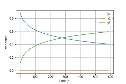
The results of the above code for different time step size is given below, the time step chosen for the calculation was 10s, 1s, 0.1s, 0.01s and 0.001s. The plots are given below, for a time step size of 10s the output is like this:

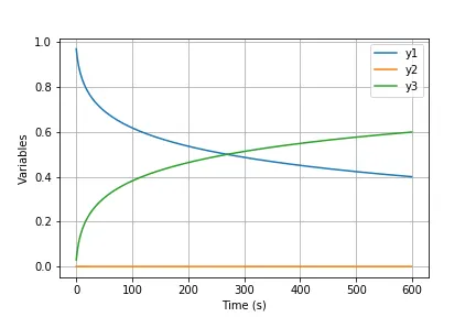
For a time step size of 1s the output is shown below:

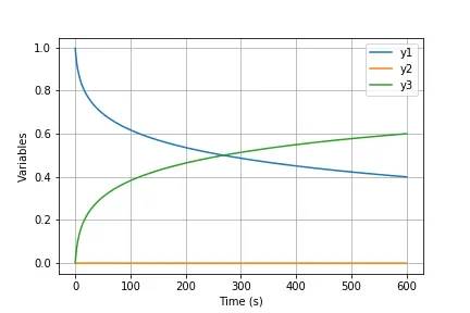
For a time step size of 0.1s the output is shown below:

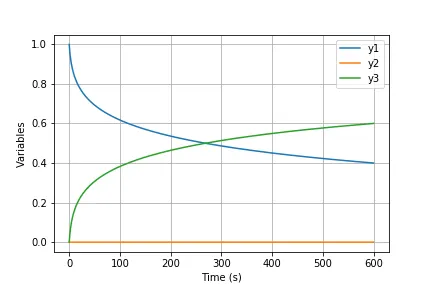
For a time step size of 0.01s the output is given below:

For a time step size of 0.001s the output is shown below:

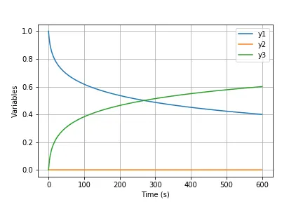
The initial value of y3 is zero so as time proceeds the value of y3 should increase but start from zero, when the time step used in the calculation is greater than 0.1 s, the value of y1 started from a value greater than zero. So the timestep that needs to be used must be very small for good calculation accuracy. 

CONCLUSION 

The code is written in python for executing the Newton-Raphson method. It is seen that when the timestep is large enough the solution is not accurate but as the time step is very less the running time is very large. It is seen that for the time step value of 0.1 the solution is becoming accurate.  So the ideal time step is set to be 0.1 s. In a stiff ODE system, the time step needs to be very small for accurate prediction of the solution.