Week 6 - Data analysis
Data visualizer (100 points)
Your script should take column numbers as the input and plot the respective columns as separate images
Each file should be saved by the name of the column
The plot labels should be extracted from the file. If, I request for a plot between column 1 (crank angle) and column 8(volume), then the label information should automatically be extracted and must appear as labels in the plots. THIS SHOULD NOT BE DONE MANUALLY.
Compatability check (30 points)
You code should exit gracefully, if a non-compatible file is provided as an input. It should say something like "File not recognized. Please provide a valid CONVERGE output file".
Basic performance calculation (50 points)
Calculate the area under the P-V diagram. P is in column 2 and V is in column 8.
Calculate the power output of this engine. Assume that RPM is 1500
This engine consumed 20 micro grams of fuel (per 1 stroke cycle). Calculate its specific fuel consumption.
Answers :
File parsing, a key technique for data extraction, is essential for making sense of and using the information hidden within different file formats. This process helps organizations unlock the full potential of their data, making it easier to understand and apply in their daily operations.
now Lets see the file parsing and data analysis using the python program coding in steps :
Python Programming...:
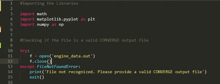
#Importing the Libraries
import math
import matplotlib.pyplot as plt
import numpy as np
#Checking if the file is a valid CONVERGE output file
try:
f = open('engine_data.out')
f.close()
except FileNotFoundError:
print('File not recognized. Please provide a valid CONVERGE output file')
exit()
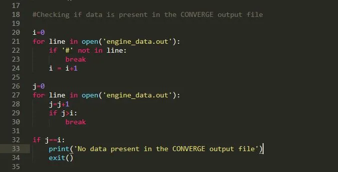
#Checking if data is present in the CONVERGE output file
i=0
for line in open('engine_data.out'):
if '#' not in line:
break
i = i+1
j=0
for line in open('engine_data.out'):
j=j+1
if j>i:
break
if j==i:
print('No data present in the CONVERGE output file')
exit()
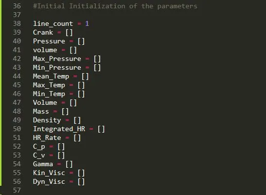
#Initial Initialization of the parameters
line_count = 1
Crank = []
Pressure = []
volume = []
Max_Pressure = []
Min_Pressure = []
Mean_Temp = []
Max_Temp = []
Min_Temp = []
Volume = []
Mass = []
Density = []
Integrated_HR = []
HR_Rate = []
C_p = []
C_v = []
Gamma = []
Kin_Visc = []
Dyn_Visc = []
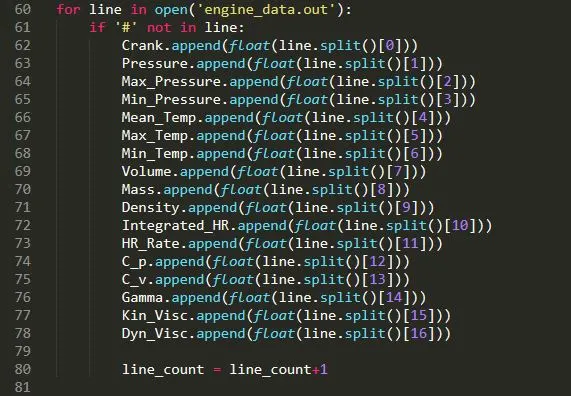
#File parsing from the data file
for line in open('engine_data.out'):
if '#' not in line:
Crank.append(float(line.split()[0]))
Pressure.append(float(line.split()[1]))
Max_Pressure.append(float(line.split()[2]))
Min_Pressure.append(float(line.split()[3]))
Mean_Temp.append(float(line.split()[4]))
Max_Temp.append(float(line.split()[5]))
Min_Temp.append(float(line.split()[6]))
Volume.append(float(line.split()[7]))
Mass.append(float(line.split()[8]))
Density.append(float(line.split()[9]))
Integrated_HR.append(float(line.split()[10]))
HR_Rate.append(float(line.split()[11]))
C_p.append(float(line.split()[12]))
C_v.append(float(line.split()[13]))
Gamma.append(float(line.split()[14]))
Kin_Visc.append(float(line.split()[15]))
Dyn_Visc.append(float(line.split()[16]))
line_count = line_count+1
#Plotting figures of parameters
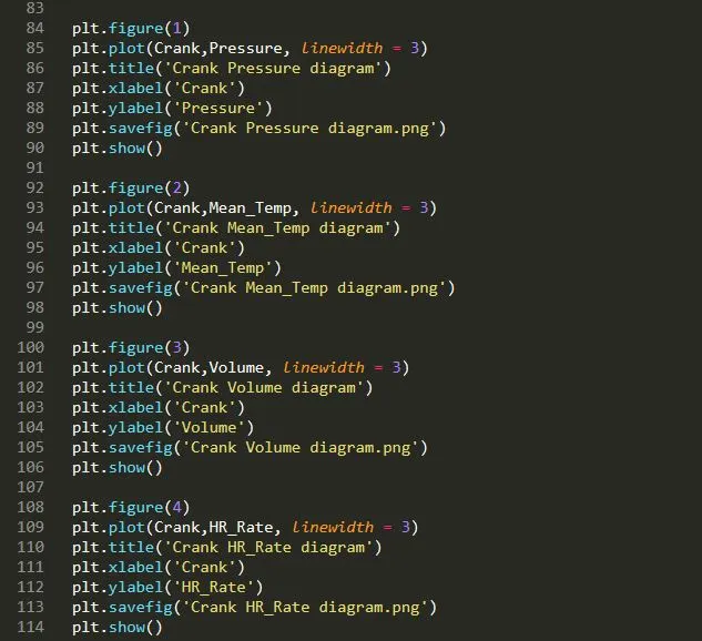
plt.figure(1)
plt.plot(Crank,Pressure, linewidth = 3)
plt.title('Crank Pressure diagram')
plt.xlabel('Crank')
plt.ylabel('Pressure')
plt.savefig('Crank Pressure diagram.png')
plt.show()
plt.figure(2)
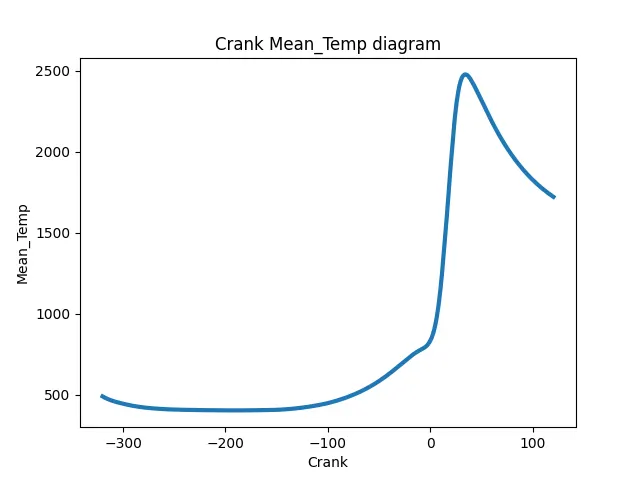
plt.plot(Crank,Mean_Temp, linewidth = 3)
plt.title('Crank Mean_Temp diagram')
plt.xlabel('Crank')
plt.ylabel('Mean_Temp')
plt.savefig('Crank Mean_Temp diagram.png')
plt.show()
plt.figure(3)
plt.plot(Crank,Volume, linewidth = 3)
plt.title('Crank Volume diagram')
plt.xlabel('Crank')
plt.ylabel('Volume')
plt.savefig('Crank Volume diagram.png')
plt.show()
plt.figure(4)
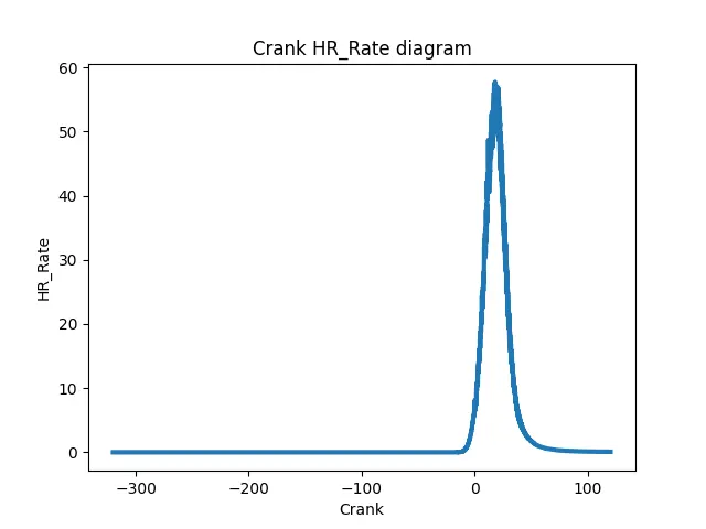
plt.plot(Crank,HR_Rate, linewidth = 3)
plt.title('Crank HR_Rate diagram')
plt.xlabel('Crank')
plt.ylabel('HR_Rate')
plt.savefig('Crank HR_Rate diagram.png')
plt.show()
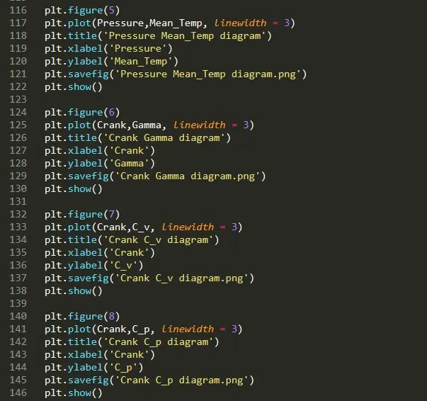
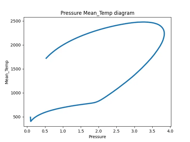
plt.figure(5)
plt.plot(Pressure,Mean_Temp, linewidth = 3)
plt.title('Pressure Mean_Temp diagram')
plt.xlabel('Pressure')
plt.ylabel('Mean_Temp')
plt.savefig('Pressure Mean_Temp diagram.png')
plt.show()
plt.figure(6)
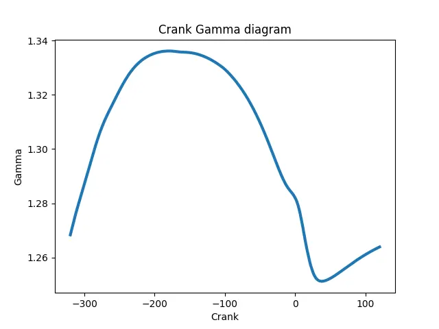
plt.plot(Crank,Gamma, linewidth = 3)
plt.title('Crank Gamma diagram')
plt.xlabel('Crank')
plt.ylabel('Gamma')
plt.savefig('Crank Gamma diagram.png')
plt.show()
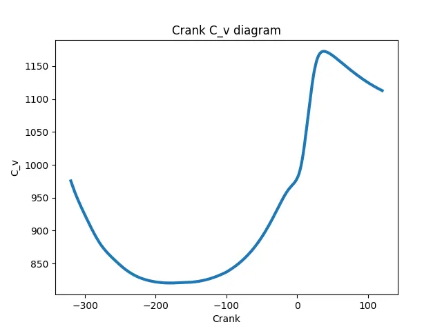
plt.figure(7)
plt.plot(Crank,C_v, linewidth = 3)
plt.title('Crank C_v diagram')
plt.xlabel('Crank')
plt.ylabel('C_v')
plt.savefig('Crank C_v diagram.png')
plt.show()
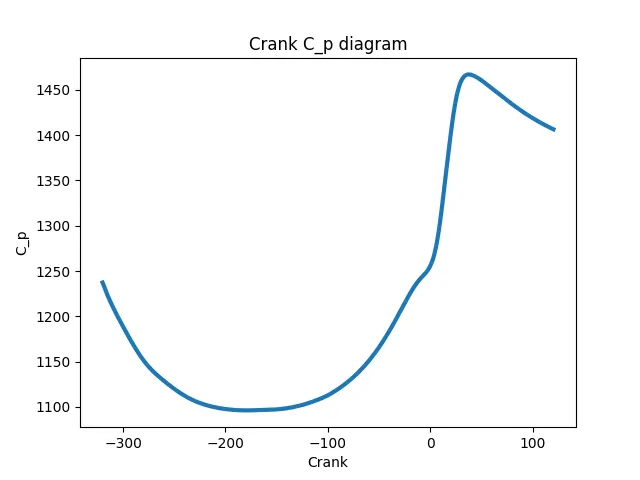
plt.figure(8)
plt.plot(Crank,C_p, linewidth = 3)
plt.title('Crank C_p diagram')
plt.xlabel('Crank')
plt.ylabel('C_p')
plt.savefig('Crank C_p diagram.png')
plt.show()
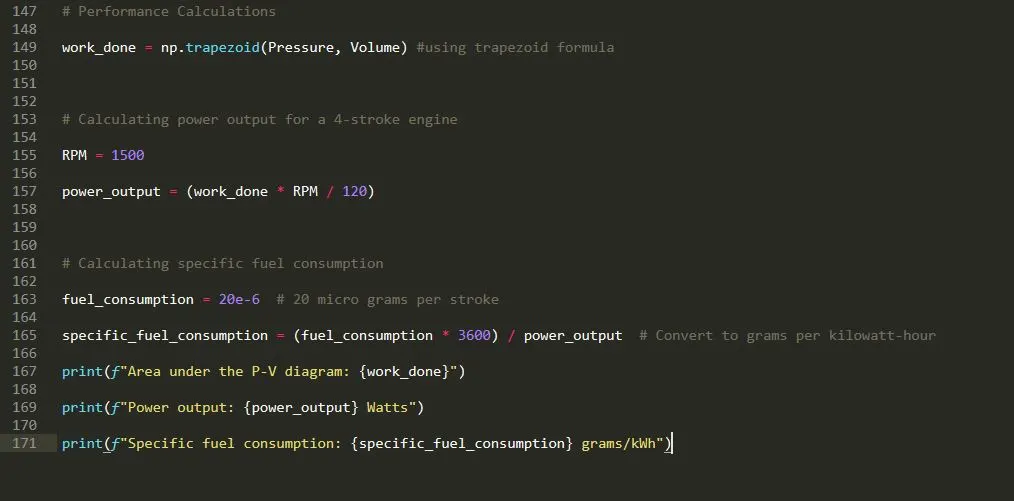
# Performance Calculations
work_done = np.trapezoid(Pressure, Volume) #using trapezoid formula
# Calculating power output for a 4-stroke engine
RPM = 1500
power_output = (work_done * RPM / 120)
# Calculating specific fuel consumption
fuel_consumption = 20e-6 # 20 micro grams per stroke
specific_fuel_consumption = (fuel_consumption * 60) / power_output # Convert to grams per kilowatt-hour
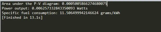
print(f"Area under the P-V diagram: {work_done}")
print(f"Power output: {power_output} Watts")
print(f"Specific fuel consumption: {specific_fuel_consumption} grams/kWh")
Step by Step program coding explaination :
step 1 :
Importing all the necessary libraries such as math, matplotlib.pyplot , numpy.
the data file is been checked whether it is available or not , if its not available then the code will show to provide a converge output file.
step 2 :
The script begins by ensuring the input file (engine_data.out) exists and contains valid data. This is crucial to prevent runtime errors caused by missing or improperly formatted files. The script attempts to open the file. If unsuccessful, it exits with an error message. The script skips commented lines (lines starting with #) and checks whether the remaining lines contain data.
step 3 :
The script assumes the file contains columns of numerical data, each representing a specific engine parameters and is stored in an empty array.
step 4 :
The data file is open and each parameters are parsed into the list for easy analysis and then the parameters are stored as a append command.
float and split is used to convert a number into the floating points and to break the line by splitting for individual values.
step 5 :
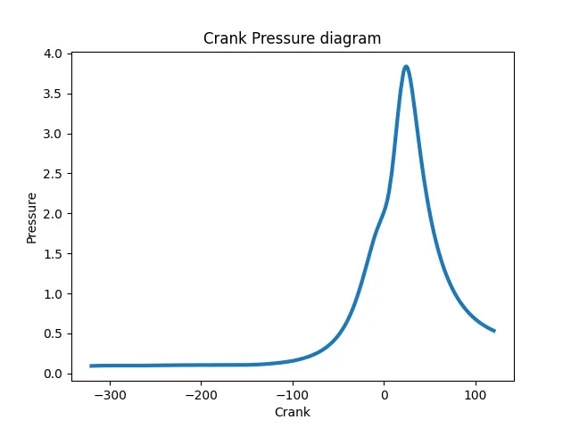
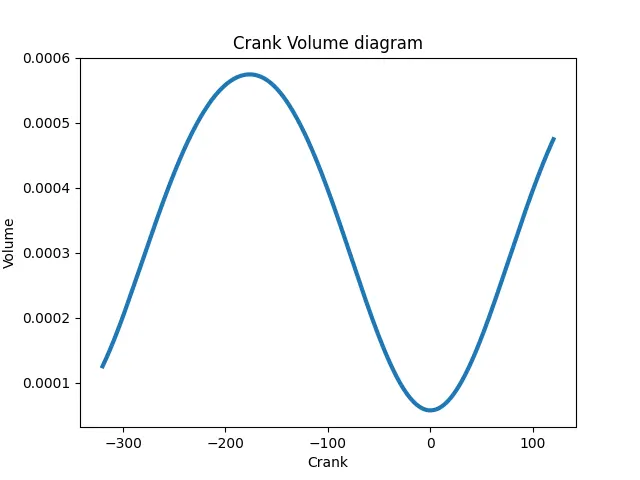
The script generates and saves plots to visualize key relationships between engine parameters:
Crank vs. Pressure: Indicates pressure variations as the crankshaft rotates.
Crank vs. Mean Temperature: Shows how cylinder temperature changes with crank angle.
Crank vs. Volume: Demonstrates the variation in cylinder volume during the cycle.
same goes with the other parameters as well.
step 6 :
Work done is been calculated the area under the P-V diagram using the trapezoidal integration method (np.trapezoid).
For a 4 stroke engine power output is been calculated by formula
power output = (Work done) / (RPM * 120) , where as RPM is given already as 1500.
Specific Fuel consumption is also been calculated for 20 micro grams per stroke fuel consumption .
Sfc = (fuel consumption * 3600)/(power output). here it is converted in 3600sec.
the output results are printed .
conclusion :
The Data from the file was parsed and executed very well and the plot are generated as well.
The performance calculations is also done
Area under the P-V diagram: 0.0005005866274680075
Power output: 0.006257332843350093 Watts
Specific fuel consumption: 11.506499942146624 grams/kWh