Challenge

Week 6 - Data analysis

SSugumar P17 Aug 2022

PYTHON

Data visualizer (100 points)

Your script should take column numbers as the input and plot the respective columns as separate images
Each file should be saved by the name of the column
The plot labels should be extracted from the file. If, I request for a plot between column 1 (crank angle) and column 8(volume), then the label information should automatically be extracted and must appear as labels in the plots. THIS SHOULD NOT BE DONE MANUALLY

Compatability check (30 points)

You code should exit gracefully, if a non-compatible file is provided as an input. It should say something like "File not recognized. Please provide a valid CONVERGE output file"

Basic performance calculation (50 points)

Calculate the area under the P-V diagram. P is in column 2 and V is in column 8.
Calculate the power output of this engine. Assume that RPM is 1500
This engine consumed 20 micro grams of fuel (per 1 stroke cycle). Calculate its specific fuel consumption.

Solution

To solve the above given problem statement, following procedure is followed:

Using a python program initally the name of the data file is taken as an input from user and checked whether the file is present or not, if the file is not pressent then the program is terminated.

Then the file is opened and data is read line by line and stored.

The name of parameters, their units and their coulmn number are stored as an array and dispalyed in form a table for the user to select the required columns.

Then the column no for independent parameter (x-axis) and dependent parameter (yaxis) is taken from user and the values of those clumn are extracted from data file and further plotted.
From the PV diagram Area under the P-V curve is calculated using the Trapezoidal Rule As we Know An area under the P-V diagram is equalto Work Done

In the next step Work was done that is calculated is used for calculating the power output

Power = Work *Speed

Specific Fuel Consumption = Mass of Fuel Consumption per hour/Power Developed in KW

IV.PYTHON PROGRAM :

import math
import numpy as np
import matplotlib.pyplot as plt

# basic initialization

line_count = 1
Crank = []
Pressure = []
Max_Pressure = []
Min_Pressure = []
Mean_Temp = []
Max_Temp = []
Min_Temp = []
Volume = []
Mass = []
Density = []
Integrated_HR = []
HR_Rate = []
C_p = []
C_v = []
Gamma = []
Kin_Visc = []
Dyn_Visc = []

#COMPATIBILITY CHECK

#Checking if the file is a valid CONVERGE output file
try:
	f = open('engine_data.out')
	f.close()
except FileNotFoundError:
	print('File not recognized. Please provide a valid CONVERGE output file')
	exit()

#Checking if data is present in the CONVERGE output file
i=0
for line in open('engine_data.out'):
	if '#' not in line:
		break
	i = i+1

j=0
for line in open('engine_data.out'):
	j=j+1
	if j>i:
		break

if j==i:
	print('No data present in the CONVERGE output file')
	exit()


# File parsing starts here
for line in open('engine_data.out'):
	if '#' not in line:
		Crank.append(float(line.split()[0]))
		Pressure.append(float(line.split()[1]))
		Max_Pressure.append(float(line.split()[2]))
		Min_Pressure.append(float(line.split()[3]))
		Mean_Temp.append(float(line.split()[4]))
		Max_Temp.append(float(line.split()[5]))
		Min_Temp.append(float(line.split()[6]))
		Volume.append(float(line.split()[7]))
		Mass.append(float(line.split()[8]))
		Density.append(float(line.split()[9]))
		Integrated_HR.append(float(line.split()[10]))
		HR_Rate.append(float(line.split()[11]))
		C_p.append(float(line.split()[12]))
		C_v.append(float(line.split()[13]))
		Gamma.append(float(line.split()[14]))
		Kin_Visc.append(float(line.split()[15]))
		Dyn_Visc.append(float(line.split()[16]))

		line_count = line_count +1


#figure
plt.figure(1)
plt.plot(Crank,Pressure, linewidth = 3)
plt.title('Crank Pressure diagram')
plt.xlabel('Crank')
plt.ylabel('Pressure')
plt.savefig('Crank Pressure diagram.png')
plt.show()

plt.figure(2)
plt.plot(Crank,Mean_Temp, linewidth = 3)
plt.title('Crank Mean_Temp diagram')
plt.xlabel('Crank')
plt.ylabel('Mean_Temp')
plt.savefig('Crank Mean_Temp diagram.png')
plt.show()

plt.figure(3)
plt.plot(Crank,Volume, linewidth = 3)
plt.title('Crank Volume diagram')
plt.xlabel('Crank')
plt.ylabel('Volume')
plt.savefig('Crank Volume diagram.png')
plt.show()

plt.figure(4)
plt.plot(Crank,HR_Rate, linewidth = 3)
plt.title('Crank HR_Rate diagram')
plt.xlabel('Crank')
plt.ylabel('HR_Rate')
plt.savefig('Crank HR_Rate diagram.png')
plt.show()

plt.figure(5)
plt.plot(Pressure,Mean_Temp, linewidth = 3)
plt.title('Pressure Mean_Temp diagram')
plt.xlabel('Pressure')
plt.ylabel('Mean_Temp')
plt.savefig('Pressure Mean_Temp diagram.png')
plt.show()

plt.figure(6)
plt.plot(Crank,Gamma, linewidth = 3)
plt.title('Crank Gamma diagram')
plt.xlabel('Crank')
plt.ylabel('Gamma')
plt.savefig('Crank Gamma diagram.png')
plt.show()

plt.figure(7)
plt.plot(Crank,C_v, linewidth = 3)
plt.title('Crank C_v diagram')
plt.xlabel('Crank')
plt.ylabel('C_v')
plt.savefig('Crank C_v diagram.png')
plt.show()

plt.figure(8)
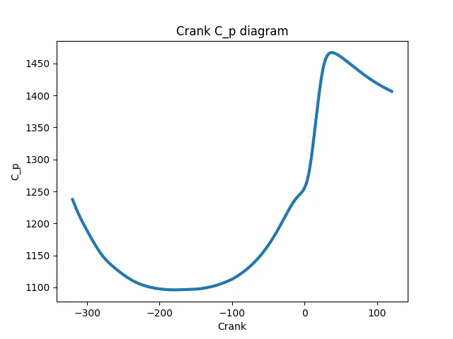
plt.plot(Crank,C_p, linewidth = 3)
plt.title('Crank C_p diagram')
plt.xlabel('Crank')
plt.ylabel('C_p')
plt.savefig('Crank C_p diagram.png')
plt.show()


# Basic performance calculation

P = 1000000*np.array(Pressure) # converting to pascal
V = np.array(Volume)

#calculating area PV diagram
AREA = np.trapz(P, V)
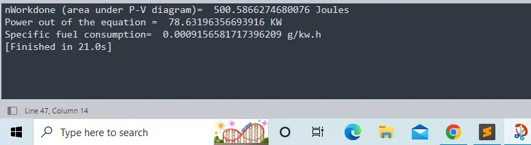
print('nWorkdone (area under P-V diagram)= ',AREA ,'Joules')

# Calculating power
power = (AREA * 2* math.pi * (1500/60))/1000
print('Power out of the equation = ',power,'KW')

#calculating specific fuel consumption
sfc = 20 * pow(10, -6)* 3600 / power
print('Specific fuel consumption= ',sfc, 'g/kw.h')

#plotting P-V Diagram
plt.figure(9)
plt.plot(Volume, Pressure, linewidth = 3)
plt.title('P-V diagram')
plt.xlabel('Volume')
plt.ylabel('Pressure')
plt.savefig('P-V diagram.png')
plt.grid()
plt.show()

Explanation:

The program can be split into 4 parts
File input and compatability check.
To get the parameter names from the data file.
To take user input to plot and save the image of two columns.
Performance calculation.

File input and compatability check

At first the required modules are imported
Then the Input command is used to ask the user to enter the file name.
Then an if loop is created to check wether the user entered file is found or not.
Which then proceeds to the compatability check.
For the data file to pass the compatability check it has to have the name 'CONVERGE' in the first line of the data.
To get the first line of the data an open variable 'titles' is created at first.
An if loop is created with the condition that if '#' in line then append the line to the empty array.
Since the first four lines of the data has '#' they get appended to the variable named 'titles'
Therefore the first index of the variable 'titles' can be used to do te compatability check.
The first index of the variable 'titles' is used in a if else loop to do the compatability check.
If the first line of the data have the name 'CONVERGE' then the program passes else exits.

Parameters of the data file

To print the parameters of the data file in the output window for the user to choose the column numbers to plot.
Now we have all the column numbers, parameters and units in the 'titles' variable
But if they are printed the way they are stored, the oder will be colapsed and also it gets printed with the '#'
So the second, third and fourth index of the 'titles' variable are given seperate for loop with some conditions and are appended to different variables.
Therefore the column number, parameters and units gets ordered which are then tabulated and printed.

Basic performance calculation

Area under the p-v curve

It can be calculated by using the simpsons method which is imported in the modules
The area is caluated using the pressure and volume variables which has the data using the simps command.
Which is then printed to the output window.
If the area is multiplied by 1e^6 then it give the work done by the engine in Joules.

To calculate the power output of the engine.

The rpm of the engine is given by the user which is used to calculate the power.
The formula used to calculate is
Power = workdone * (strokecycle/1000) KW
Workdone = area*1e6
strokecycle = rps/2
By using the above formula the power of the engine is calculated for the given rpm.

To calculate the specific fuel consumption.

The fuel consumption of the engie per stroke in mili grams is taken as input from the user
Which is then used to calculate the specific fuel consumption using the formula

BSFC = r/P
where, BFSC - Brake specific fuel consumption (g/J)
r - fuel consumption rate in grams per second (g/s)
P - Power output of the engine (W)
BSFC [g/(kW⋅h)] = BSFC [g/J] × (3.6 × 10⁶)
BSFC [g/(kW⋅h)] = BSFC [mg/KW] × (3.6)

Using the above formula the BSFC is calculated. The units are converted accordingly.

At the end of the code a choice is given to the user wether to continue or end the program which is done using a while loop. A variable 'x' with value 1 is used for the condition. If the user wish to continue to plot and save multiple images then the x = 1 condition is to be maintained by the user. If the value of the x variable is change then the program ends.

VI. RESULTS :

figure 1

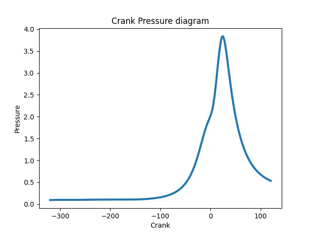
figure 2

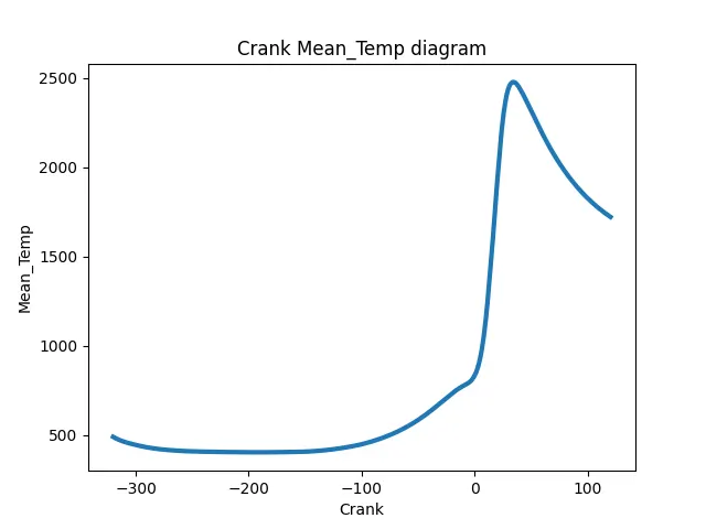
figure 3

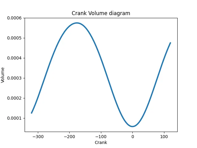
figure 4

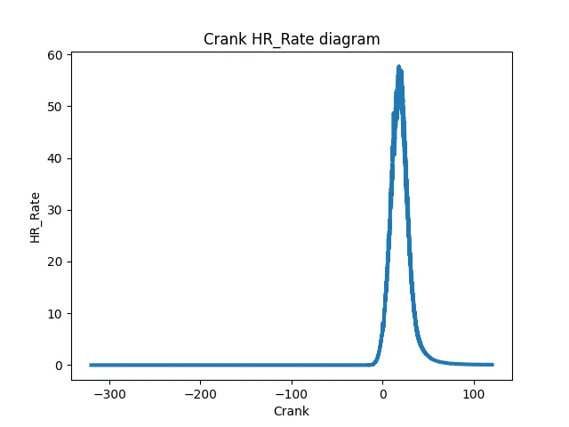
figure 5

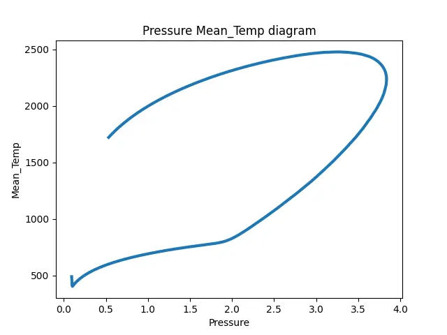
figure 6

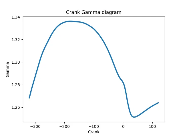
figure 7

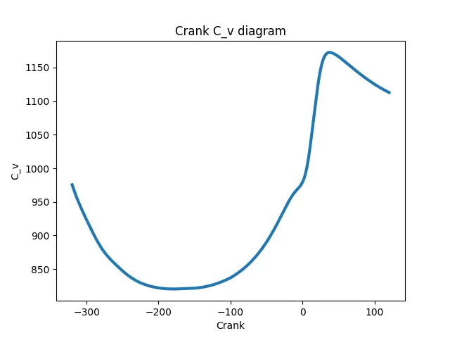
figure 8

Basic performance calculation (50 points)

Calculate the area under the P-V diagram. P is in column 2 and V is in column 8.
Calculate the power output of this engine. Assume that RPM is 1500
This engine consumed 20 micro grams of fuel (per 1 stroke cycle). Calculate its specific fuel consumption.

Area under the p-v curve

It can be calculated by using the simpsons method which is imported in the modules
The area is caluated using the pressure and volume variables which has the data using the simps command.
Which is then printed to the output window.
If the area is multiplied by 1e^6 then it give the work done by the engine in Joules.

To calculate the power output of the engine.

The rpm of the engine is given by the user which is used to calculate the power.
The formula used to calculate is
Power = workdone * (strokecycle/1000) KW
Workdone = area*1e6
strokecycle = rps/2
By using the above formula the power of the engine is calculated for the given rpm.

To calculate the specific fuel consumption.

The fuel consumption of the engie per stroke in mili grams is taken as input from the user
Which is then used to calculate the specific fuel consumption using the formula

BSFC = r/P
where, BFSC - Brake specific fuel consumption (g/J)
r - fuel consumption rate in grams per second (g/s)
P - Power output of the engine (W)
BSFC [g/(kW⋅h)] = BSFC [g/J] × (3.6 × 10⁶)
BSFC [g/(kW⋅h)] = BSFC [mg/KW] × (3.6)

Using the above formula the BSFC is calculated. The units are converted accordingly.

Output

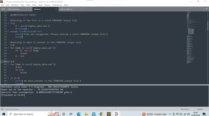
Along with these program second figure of plot in common is PV diagram:

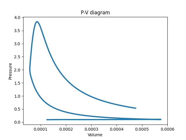
The data from the output file was read successfully and the plot required as per the user need was made.

The performance calculations were done and displayed successfully.

Workdone (area under P-V diagram)= 500.5866274680076 Joules

Power out of the equation = 78.63196356693916 KW

Specific fuel consumption= 0.0009156581717396209 g/kw.h

Main Window

Week 6 - Data analysis

Ship work like this
in your own course.

Talk to a career counsellor

Ship work like thisin your own course.

Talk to a career counsellor

Ship work like this
in your own course.