Challenge

Week 6 - Data analysis

HHarsh Shah22 Sept 2020

AIM:- VISUALIZE DATA IN PYTHON FROM A LARGE DATASET PROVIDED FROM THE DATA FILE

THEORY:-

Data visualization is a tool that can be used to pictorially represent how particular parameters behave , their relations by means of graphs, charts etc.

Python has extensive capabilities to visualize data in the aforementioned manner.

Now we have been provided an external data file which contains simulation results of an engine for which the dataset looks something like this:

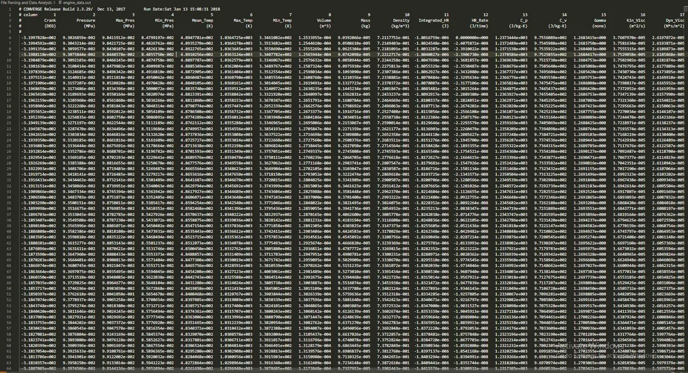Fig(1) - Simulation data

Now if we want to ascertain at a certain crank angle what are the other parameters affected, data visualization comes as a handy tool.

Also if we want to study certain areas of interest in specific parameters, visualizing the data will be useful.

So we try to visualize data using PYTHON programming language meanwhile also getting the idea of python's file I/O capabilities, exception handling, plotting etc.

SOLUTION:-

PROGRAM:-

''' File parsing - Data visualizer
      Author: Harsh J Shah'''

#Importing libraries
import matplotlib.pyplot as plt
import math
import numpy as np

# Checking file compatibility
try:
    file_name = open('engine_data.out')
except: 
    print("'File not recognized. Please provide a valid converge output file'")

# INITIALIZE counter and empty arrays
line_ct = 0
x = []
y = []

# SELECCTION OF PARAMETERS AND PROVIDING INPUT
print("Please select parameters for the plot below:")
print(""" 
	 00-\t\t01-Crank\t02-Pressure\t 
	 03-Max_Pres\t04-Min_Pres\t05-Mean_Temp 
	 06-Max_Temp\t07-Min_Temp\t08-Volume 
	 09-Mass\t\t10-Density\t11-Integrated_HR 
	 12-HR_Rate\t13-C_p\t\t14-C_v 
	 15-Gamma\t16-Kin_Visc\t17-Dyn_Visc\n""")
			
col_x = int(input('Please select the parameter for x-axis by specifying the parameter number:')) - 1
col_y = int(input('Please select the parameter for y-axis by specifying the parameter number:')) - 1 


# EXTRACTING THE DATA
for line in file_name:	
    if '#' not in line:
	x.append(float (line.split()[col_x]))
	y.append(float (line.split()[col_y]))


# ARRAY FOR LABELLING
z = ['Crank(DEG)', 'Pressure(MPa)', 'Max_Pres(MPa)', 'Min_Pres(MPa)', 'Mean_Temp(K)', 'Max_Temp(K)', 'Min_Temp(K)', 'Volume(m^3)', 
'Mass(kg)', 'Density(kg/m^3)', 'Integrated_HR(J)', 'HR_Rate(J/time)', 'C_p(J/kg-K)', 'C_v(J/kg-K)', 'Gamma(none)', 'Kin_Visc(m^2/s)', 'Dyn_Visc(N*s/m^2)']

#PLOTTING WITH AUTOMATED LABELLING
plt.plot(x,y)
plt.xlabel(z[col_x])
plt.ylabel(z[col_y])
plt.grid()
plt.show()


# ENGINE PERFORMANCE PARAMETERS CALCULATION

if col_x == 7 and col_y == 1:
   integrate_curve = np.trapz(y,x)
   rpm = 1500
   print("The RPM at which the engine performance is calculated is:", rpm)
   
   # CALCULATING WORK DONE
   work = integrate_curve * 1e6
   print('The work done by the engine at specified RPM represented by the area under the P-V plot is:', work, 'J')
	
   # CALCULATING POWER OUTPUT BY THE ENGINE
   power_output = (rpm * work)/(60 * 1000 * 2)
   print ('The power output by the engine at specified RPM is:', power_output,'kW')
	
   # CALCULATING SPECIFIC FUEL CONSUMPTION
   fuel_per_stroke = 20 * pow(10,-9) 
   fuel_per_second = fuel_per_stroke * (rpm/60)*0.5
   fuel_per_hour = fuel_per_second * 3600
   sfc = fuel_per_hour/power_output
   print('The specific fuel consumption of the engine at specified RPM is:',sfc,'kg/(kW-hr)')

# Closing the file
file_name.close()

SECTION 1: IMPORTING LIBRARIES

#Importing libraries
import matplotlib.pyplot as plt
import math
import numpy as np

Required libraries like numpy, matplotlib, math were imported.

SECTION 2: CHECKING FILE COMPATIBILITY

# Checking file compatibility
try:
	file_name = open('engine_data.out')
except: 
	print("'File not recognized. Please provide a valid converge output file'")

We open the file using open command which is a feature of python's file handling capability. As soon as we open the file we can provide certain attribute like reading, writing, appending data from the file.

Default is set to read mode. In case its needed to be specified we can specify it in follwing manner:

open('engine_data.out', 'r')

Its noteworthy that the file must be in the same location where the program is going to be saved and the characters of filename must be asme as psecifed in the open command.

When the file is not in the same location as the Program or characters of filename are mismatching it generates an error which is known as I/O error.

Now sometimes mistakes like this may disrupt the normal flow of the program which is termed as exception event.

If you have some disruptive code that may raise an exception, you can defend your program by placing the suspicious code in a try: block. After the try: block, include an except: statement, followed by a block of code which handles the problem as elegantly as possible.

Thats what has been used here to check for the file compatibility.

SECTION 3: INTIALIZATION OF COUNTER AND EMPTY ARRAYS. SPECIFYING PARAMETERS FOR PLOT ON X AND Y AXIS.

line_ct = 0
x = []
y = []

print("Please select parameters for the plot below:")
print(""" 
	 00-\t\t01-Crank\t02-Pressure\t 
	 03-Max_Pres\t04-Min_Pres\t05-Mean_Temp 
     06-Max_Temp\t07-Min_Temp\t08-Volume 
	 09-Mass\t\t10-Density\t11-Integrated_HR 
	 12-HR_Rate\t13-C_p\t\t14-C_v 
	 15-Gamma\t16-Kin_Visc\t17-Dyn_Visc\n""")
			
col_x = int(input('Please select the parameter for x-axis by specifying the parameter number:')) - 1
col_y = int(input('Please select the parameter for y-axis by specifying the parameter number:')) - 1

Initialized line counters and empty array x and y for storing plot parameters. The multiple plot parameters were stored as strings in multiple lines using """ thrice.

col_x and col_y take numeric integers values clearly indicated by the int specified and input requests the user to provide a input.

SECTION 4: EXTRACTION OF DATA

for line in file_name:	
    if '#' not in line:
	x.append(float(line.split()[col_x]))
	y.append(float(line.split()[col_y]))

Now to read lines and extract the data into respective arrays we use a for loop which reads every line of the data file.

But some lines do contain irrelevant data like strings which are parameter names which will cerate an issue while plotting the data.

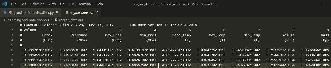
FIG(2) - IRRELEVANT LINES FOR PLOT

Now from FIG(2); we can clearly say that lines 1-5 will create an error while generating plot for parameters. So we specify if there is no # in that line consider that line for appendingthe values in the empty array.

x.append(float(line.split()[col_x]))

We add the values of our interested parameters as every line is and the split command splits the strings by the specified seperator which is a whitespace in our case. Now as this sis read like a string we need toconvert to float so we specify a float command which shall convert the string to numeric values so that it can be used for plotting.

col_x is specified to index the whole column with the parameter considered for x- axis. Similar is the case for y-axis. Now here there is a reason justfied for specifying value for col_x = parmater no - 1. Because python generally considers values from zero. So crank will be at a position of column zero but while passing it as the parameter if we specify 1 the values for pressure will be taken for plotting.

SECTION 5: PLOTTING AND AUTOMATED LABELLING

z = ['Crank(DEG)', 'Pressure(MPa)', 'Max_Pres(MPa)', 'Min_Pres(MPa)', 'Mean_Temp(K)', 'Max_Temp(K)', 'Min_Temp(K)', 'Volume(m^3)', 
'Mass(kg)', 'Density(kg/m^3)', 'Integrated_HR(J)', 'HR_Rate(J/time)', 'C_p(J/kg-K)', 'C_v(J/kg-K)', 'Gamma(none)', 'Kin_Visc(m^2/s)', 'Dyn_Visc(N*s/m^2)']

plt.plot(x,y)
plt.xlabel(z[col_x])
plt.ylabel(z[col_y])
plt.grid()
plt.show()

z is an array consisting of parameters as the strings which can be used for labelling the plot automatically on the basis of inputs we provide.

Here also note that we start with zero so that the input that we have provided as parameter for x and y -axis matches the same array value so that it cna be accessed directly as per the speicified paramter

Suppose we provide x-axis parameter as 08 i.e.Volume

y- axis parameter as 02 i.e. Pressure. Our inputs will be 08 and 02.

col_x will be 7 and col_y will be 1.

Now as python starts reading from zero it will read pressure values at position - 1 and volume values at position - 7

So when we index for label from z array we can see that the value position are directly corresponding to col_x and col_y values.

Section 6: CALCULATING ENGINE PERFORMANCE PARAMETERS

if col_x == 7 and col_y == 1:
   integrate_curve = np.trapz(y,x)
   rpm = 1500
   print("The RPM at which the engine performance is calculated is:", rpm)
   work = integrate_curve * 1e6
   print('The work done by the engine at specified RPM represented by the area under the P-V plot is:', work, 'J')
   
   power_output = (rpm * work)/(60 * 1000 * 2)
   print ('The power output by the engine at specified RPM is:', power_output,'kW')
   
   fuel_per_stroke = 20 * pow(10,-9) 
   fuel_per_second = fuel_per_stroke * (rpm/60)*0.5
   fuel_per_hour = fuel_per_second * 3600
   sfc = fuel_per_hour/power_output
   print('The specific fuel consumption of the engine at specified RPM is:',sfc,'kg/(kW-hr)')

Now, we will take a look at how the data can be used to compute certain performing characteristics of the component.

We have been provided certain input parameters like rpm, fuel per stroke.

Calculating work done:- It can be calculated by integrating the pressure - volume curve. Units need to be taken care of as it is MPa we multiply by `10^6` to maintain th units at Pascals.

But how is the pressure -volume plot integrated?

Python has inbuilt function trapz from the numpy module which used trapezoidal rule to integrate the values under a given plot.

Calculating Power output:-

From P-V plot we can clealry say that this is a 4 stroke engine. ASSUME THE NO OF CYLINDER TO BE 1

for which `Power = (RPM * WORK DONE)/(60 * 1000 * 2)`

REVOLUTIONS PER SECOND:- `RPS = (RPM)/60`

CYCLES PER SECOND = RPS/2 (for a 4 stroke engine)

Since we computed work done in Joule so we divide by 1000.

Calculating Specific fuel consumption:-

sfc = (fuel consumed in kg per hr)/(power (kW)

We have been provided 20 micrograms of fuel per stroke cycle

So `20 * 10^-9` is kg of fuel per stroke cycle

fuel consumed per second = fuel per stroke cycle * rps/2

fuel consumed per hour = fuel consumed per second * 3600 seconds

Section 7: Closing the file

file_name.close()

The close command closes the data file.

PLOTS AND RESULTS:-

The P-V plot is as follows:-

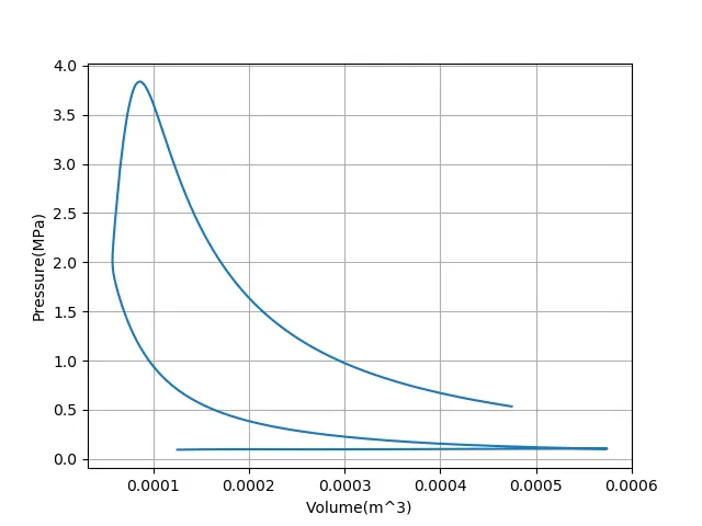
FIG (3) - PV PLOT

OUTPUT FOR ENGINE PERFORMANCE CHARACTERISTICS:-

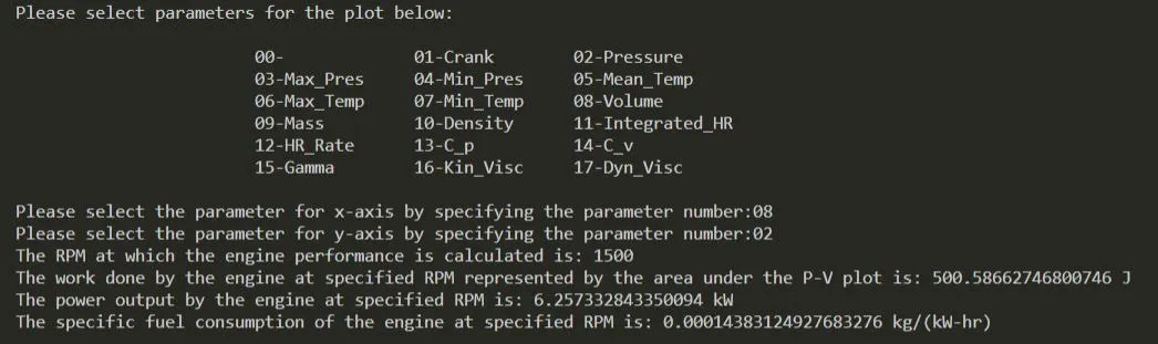
FIG (4) - OUTPUT

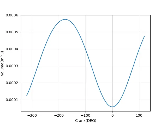
The Volume - crank angle plot is as follows:-

CONCLUSION:-

We can clearly infer that data visualization can be a very rich tool to assess how parameters are affected, what is their relation, how they behave and can help in assessing our certain areas of interest.

Thank you.

Week 6 - Data analysis

Ship work like this
in your own course.

Talk to a career counsellor

Ship work like thisin your own course.

Talk to a career counsellor

Ship work like this
in your own course.