Week 5 - Curve fitting
AIM:- Generate a curve fit plot for Specific heat (`C_p`) vs Temperature (`T`) using a linear and a cubic model.
THEORY:-
A set of data points are available with us which are plotted as points in the co-ordinate system as shown in the figure below.
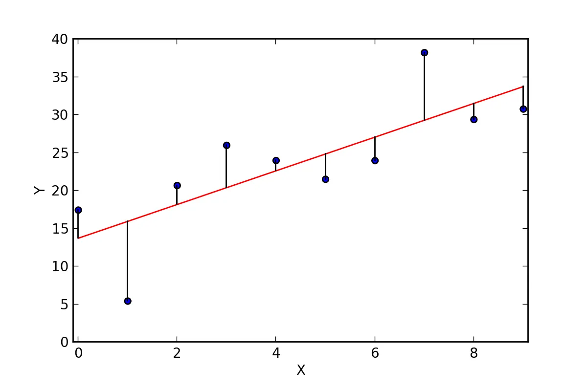
FIG (1) - SAMPLE CURVE FIT PLOT
Curve fitting is a numerical technique which helps to find the best possible fit for the dataset available with us. It is an approximate technique and is suitable to linear as well as higher order polynomial equations also.
The technique computes the co-efficient in the equation models where one function is dependent on the other function.
This application of curve fitting helps to determine how a function behaves in response to a certain parameter i.e helps to generate an appropriate mathematical model of the data provided.
It does not have applications limited to engineering only but can be applied to social sciences, market behaviour (finances), psychology, natural proceeses for a given set of data.
SOLUTION:-
We have been provided with a set of values for temperature and specific heat from the data file.
A linear and cubic model will be used to generate the best suitable fit for the data or simply the model will try to emulate the original dataset.
Linear model is represented by `y = ax + b` whereas cubic model is represented as`y = ax^3 + bx^2 + cx + d`. In both the cases x is the independent variable and y is the dependent one.
In our case the dependent variable is specific heat (`C_p`) and the temperature (`T`) is the independent one.
A code was written in Python and curve fitting was performed using curve_fit function from the scipy.optimize model.
The curve_fit function computes the co-efficients ( a, b in linear model and a,b,c,d in cubic model) and then for specific temperature value it calculates the value of specific heat using the model equations.
PROGRAM:-
# Curve fitting
# Author: Harsh Shah

# Importing Required Libraries
import numpy as np
import matplotlib.pyplot as plt
import math
from scipy.optimize import curve_fit
from prettytable import PrettyTable

# Defining Linear and cubic polynomials
def linear(t,a,b):
    return a*t+ b

def cubic(t,a,b,c,d):
    return a*pow(t,3)+ b*pow(t,2) + c*t + d


# Extracting values from data set
def read_file():
    temperature=[]
    cp=[]
    for line in open('data','r'):
	values = line.split(',')
	temperature.append(float(values[0]))
	cp.append(float(values[1]))
    return [temperature, cp]

temperature,cp = read_file()

# Perform Curve fit using curve_fit
popt_l, pcov_l = curve_fit(linear, temperature, cp)
popt_c, pcov_c = curve_fit(cubic, temperature, cp)

# Computing specific heat values as per the curve_fit functtion
fit_cp_l = linear(np.array(temperature), *popt_l)
fit_cp_c = cubic(np.array(temperature), *popt_c)

# Plotting
plt.plot(temperature, cp, color='blue', linewidth = '2')
plt.plot(temperature, fit_cp_l, color='red', linewidth = '2')
plt.plot(temperature, fit_cp_c, color='green', linewidth = '2')
plt.legend(['Actual data','Linear fit','Cubic Fit'])
plt.xlabel('Temperature [K]')
plt.ylabel('Cp')
plt.grid()
plt.show()

#Calculating mean of Specific heat Cp
mean_cp = sum(cp)/len(cp)

# Calculating sum of squares of regression for linear fit
reg_lin = []
for cp_lin in fit_cp_l:
    z = pow((cp_lin - mean_cp),2)
    reg_lin.append(z)
ssr_lin = sum(reg_lin)

# Calculating sum of squares of error for linear fit
err_lin = []
for j,k in zip(fit_cp_l,cp):
    z = pow((j - k),2)
    err_lin.append(z)
sse_lin = sum(err_lin)

#Calculating SST for linear fit
sst_lin = ssr_lin  + sse_lin

#Calculating R square for linear fit
r_square_lin = ssr_lin/sst_lin

#Calculating Root mean square value for linear fit
RMSE_lin = math.sqrt(sse_lin/len(cp))

# Calculating sum of squares of regression for cubic fit
reg_cubic = []
for cp_cubic in fit_cp_c:
    z = pow((cp_cubic - mean_cp),2)
    reg_cubic.append(z)
ssr_cubic = sum(reg_cubic)

# Calculating sum of squares of error for cubic fit
err_cubic = []
for j,k in zip(fit_cp_c,cp):
    z = pow((j - k),2)
    err_cubic.append(z)
sse_cubic = sum(err_cubic)

#Calculating SST for cubic fit
sst_cubic = ssr_cubic  + sse_cubic

#Calculating R square for cubic fit
r_square_cubic = ssr_cubic/sst_cubic

#Calculating Root mean square value for cubic fit
RMSE_cubic = math.sqrt(sse_cubic/len(cp))

# Generating tabular values for linear fit
table_l = PrettyTable(["Cp mean", "SSR", "SSE", "SST", "R-SQUARE", "RMSE"])
table_l.add_row([mean_cp, ssr_lin, sse_lin, sst_lin, r_square_lin, RMSE_lin])
print("For linear fit: \n", table_l)

# Generating tabular values for cubic fit
table_c = PrettyTable(["Cp mean", "SSR", "SSE", "SST", "R-SQUARE", "RMSE"])
table_c.add_row([mean_cp, ssr_cubic, sse_cubic, sst_cubic, r_square_cubic, RMSE_cubic])
print("For cubic fit: \n", table_c)
Code Analysis:-
1. Importing library: numpy, matplotlib.pyplot, scipy.optimize for using curve_fit function, math library and pretty table library to generate tables for results.
2. Defining function: Linear and cubic equations are defined using functions.
3. Reading file: Our dataset the temperature and specific heat values are extracted and stored in empty arrays of temperature and specific heat. We need to extract or read values one by one and store the in their designated array. So similar to reading a book, we first need to open it here; open function was used to open the file named 'data' which is the 1st parameter and after opening it we need to read it so 'r' was passed as the 2nd parameter.
Now, as we need to read the file line by line a for loop is used and as the values were seperated in the data file by a comma (,) so a split command was specified to segregate the values in two parts and store them in the designated arrays.
4. Perform curve fit and plot:
Curve fitting is done by curve_fit function imported from scipy.optimize module.
The function requires following arguments:
- Model function: whether linear, quadratic, cubic, higher order polynomials etc. Here we call linear and cubic model functions in our case.
- Independent variable: Temperature is specified in our case as we have defined the model equation with temperature being the parameter to output the value of specific heat.
- Dependent variable: Specific heat varies on basis of temperature value.
The curve fit function outputs two values popt and pcov where popt is the value of co-efficients computed by the curve fit function.
Now using our computed co-efficient values from curve_fit command and independent variable i.e. temperature values we calculate values for specific heat CP .
This newly calculated Cp values are plotted against their corresponding Temperature values on a Cartesian co-ordinate system. The plot for the original data set and computed values can then be compared to evaluate the fit whether it is better or bad.
5. Calculating statistical paramters like mean Cp, SSR (sum of squares of regression), SSE (sum of square of errors), SST, R-square, Root mean square values (RMSE) and tabulating the results. This statistical parmaters help us evaluate whehter the fit is better or not.
PLOT AND RESULTS:-
The output plots for the program were as follows:-
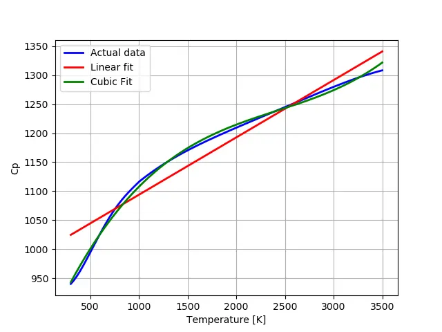
Fig(2)- Linear and cubic fit plot with the dataset plot
On visual inspection we can clearly say that cubic fit is much more a better fit than linear fit as it tries to emulate the behaviour of original dataset as closely possible.
The statistical parameter output values are as shown in the image below:
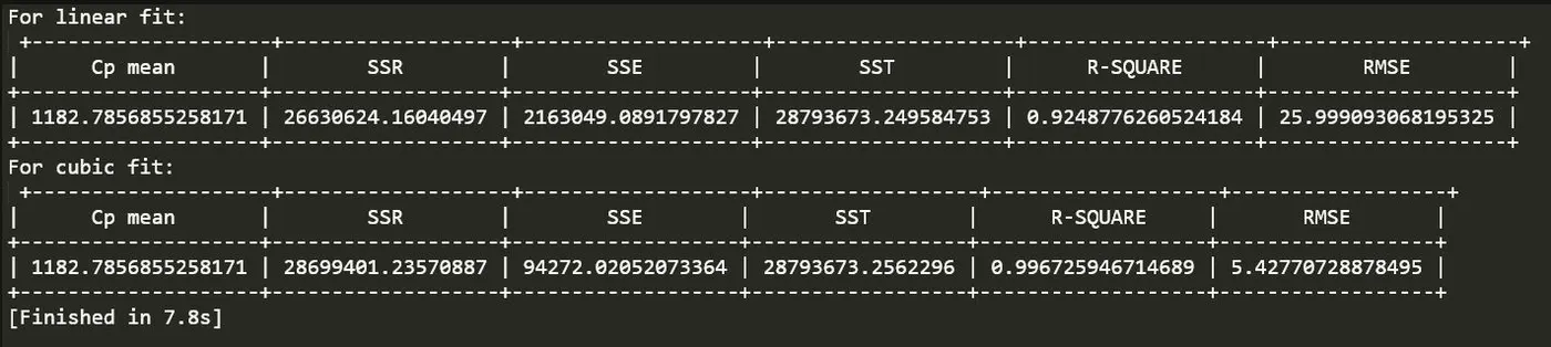
Fig(3)- Statistical parameter output values
Questions:-
Q1. What does popt and pcov mean?
Sol:- popt is the output array which stores the values for co-efficients of the linear and cubic models we have defined.
pcov is the co-variance of the co-efficient vlaues.
Q2. What does np.array(temperature) do?
Sol:- It creates a temperature array that can be used for model functions defined by us
Q3. What does the * in *popt mean?
Sol:- fit_cp_l = linear(np.array(temperature), *popt_l)
Here we call the earlier defined linear function which requires input as t which we provide as the temperature array and a and b are the co-effficients computed by the curve_fit function and stored in the popt_l array.
The * refers to access the co-efficients from popt array and multiply them with temperature values obtained from temperature array and compute new values for specific heat (`C_p`)
Q4. Write code to fit a linear and cubic polynomial for the Cp data. Explain if your results are good or bad.
Sol:- Refer Solution, Program and Plot and result section.
Q5. What needs to be done in order to make the curve fit perfect?
Sol:- Perfect is very rarely possible but it can be made better by using higher order polynomials or splitting the dataset over intervals and applying different models to specific intervals.
Q6. Show empirically as to how well your curve has been fit.
Sol:- Formulating the equations for Sum of Squared Errors (SSE), R square and RMSE.
`R^2 = (SSR)/(SST)`
where SST = SSR + SSE.
SSR represents sum of squares of regression and SSE represents sum of squares of error.
SSR (sum of squares of regression) is the sum of squares of difference between estimated values of dependent variable and the mean of dependent variable from original dataset.
In our case,`SSR = sum_(i=1)^n (predicted C_p - mean Real C_p)^2`
SSE (sum of squares of error) is the sum of squares of difference between estimated values and original values of the real dataset.
`SSE = sum_(i=1)^n (Estimated C_p - real C_p)^2`
Root mean square error provides a standard deviation of any random point in the dataset.
`RMSE = sqrt((SSE)/n)` where n represetns the number of elements in the datatset.
Generally for curve fits; `R^2` greater than 0.95 is desired for better fits. [Ref 1].
Lower values of RMSE indicate a good fit. RMSE is a good measurement of how accurately our model (i.e assumed polynomial) predicts the response. [Ref 3]
All the above mentioned Parameters were calculated for linear as well as cubic fit and shown in fig (3).
REFERENCES:-
1. https://projects.skill-lync.com/projects/Curve-Fitting-and-criterion-to-choose-best-fit-41860
2. https://www.geeksforgeeks.org/python-programming-language/
3. https://in.mathworks.com/help/matlab/ref/polyfit.html
4. https://docs.scipy.org/doc/scipy/reference/generated/scipy.optimize.curve_fit.html
THANK YOU.