Conjugate Heat Transfer Simulation

Introduction

CHT or conjugate heat transfer, refers to a heat transfer process involving an interaction of conduction within a solid body and the convection between the moving liquid media and solid media. Heat transfer in the solid domain is primarily due to conduction, for the fluid domain, it is dominated by convection. The heat transfer from one media to other, depends upon the fluid particles velocity to some extent.

There is a wide range of application of the CHT phenomenon, most primarily in cooling applications. A wide variety of active as well as passive cooling systems is employed around the heat producing electric or mechanical component, that works on CHT phenomenon. One of the common live examples around us is fins for circuit board, using natural convection or passive cooling.

CHT analysis plays a crucial role in determining the products design. As a rule of thumb, increased surface area leads to faster cooling, but the exact dimensions have to be simulated in order to be applied effectively. CHT analysis is very handy and important method with which can calculate the design parameters and reveal important data points before experimentation.

CHT analysis with a propriety software (CONVERGE CFD) is the subject of present study.

Super Cycling

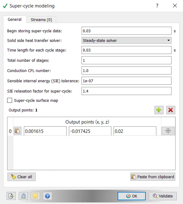
In Converge CFD, the solution of different medium cannot be solver at same speed. The solution for liquid is much fast than solution of conduction in solid. In order to remove the much difference of temperature at interface and for easy convergence, super cycling is introduced. The time interval for super cycling signifies that, the fluid solver should be stopped and wait till the solid conduction reaches steady state.

Objective

To run a baseline simulation CHT simulation, of a flow inside a pipe. Heat is given from outside the pipe.

To simulate the grid independence test.

To study the effect of super cycling.

Outline

The study has been carried out in 2 steps. In the first step grid independence test has been done using 3 different grid sizes. In the second step effect of super cycling has been studied using the most computationally efficient grid.

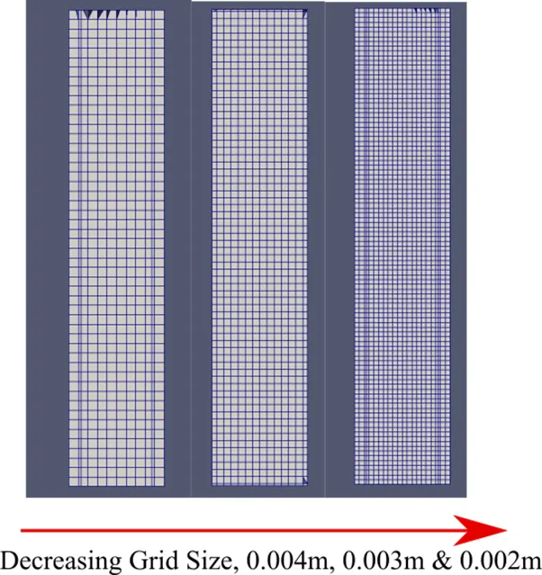
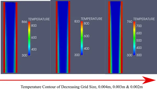
Grid Independence Study has been carried out with the grid size of 0.004m, 0.003m and 0.002m

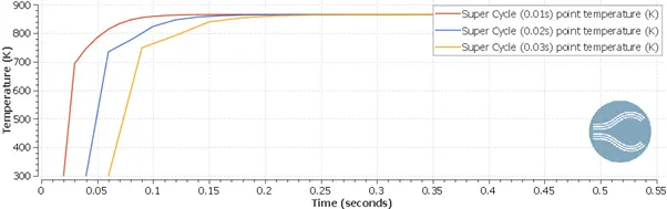
Effect of super cycling has been studied with the interval of 0.01s, 0.02s, and 0.03s.

Simulation

Geometry

The geometry with named boundary has been given below. The total length of piper is 0.2m.

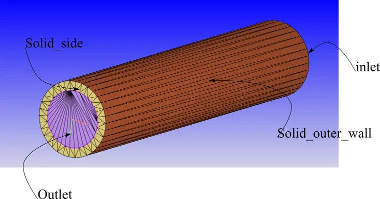
Boundary

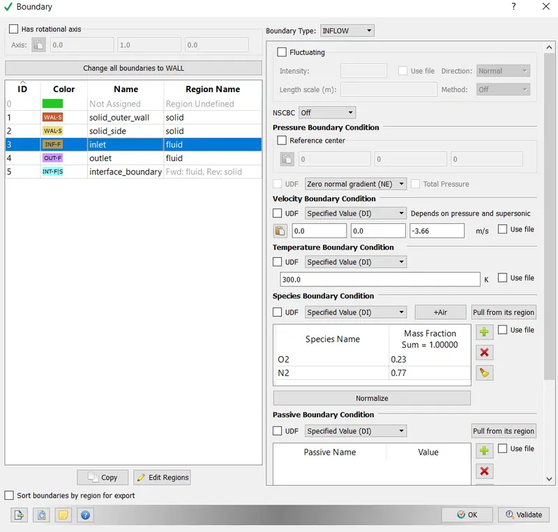
inlet

outlet

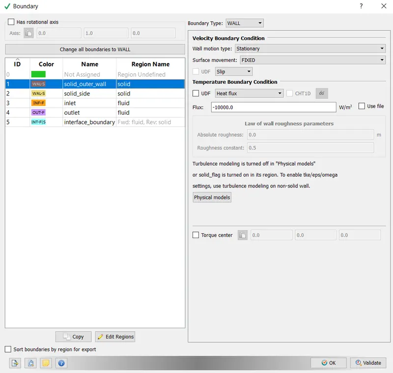
outer wall

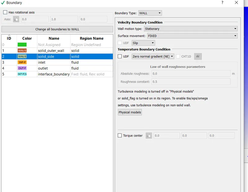
solid side

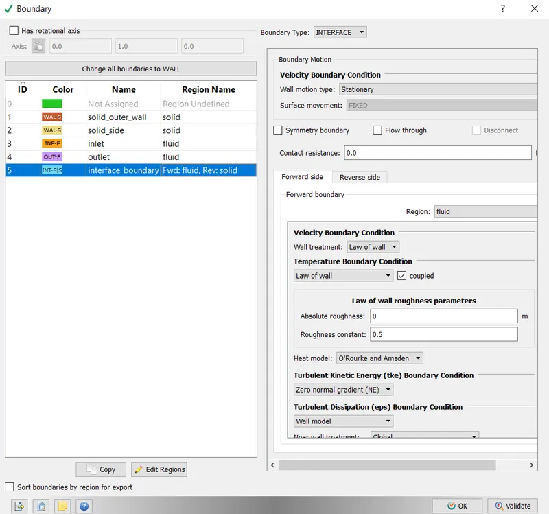
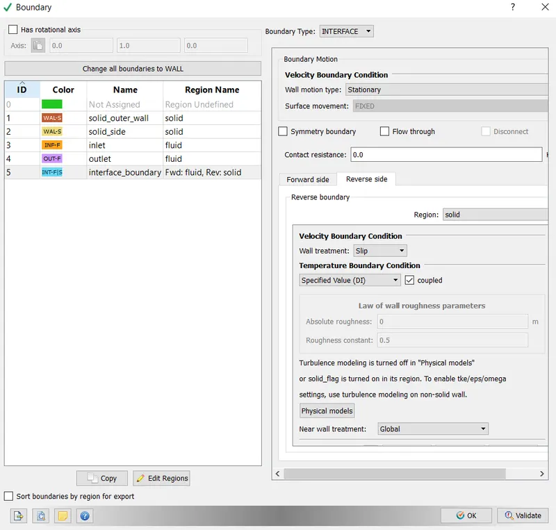
interface

forward

reverse

Initial Conditions

Simulation Parameters

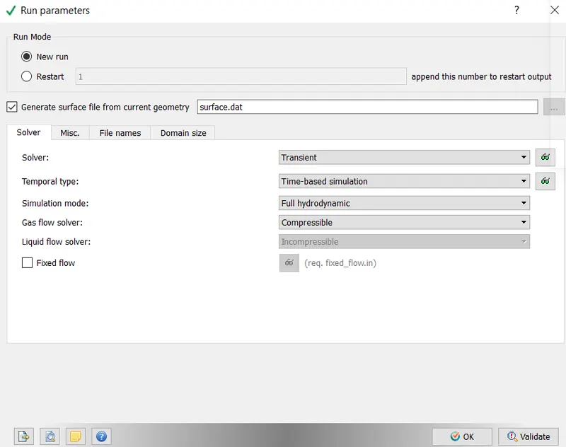
Run Parameters

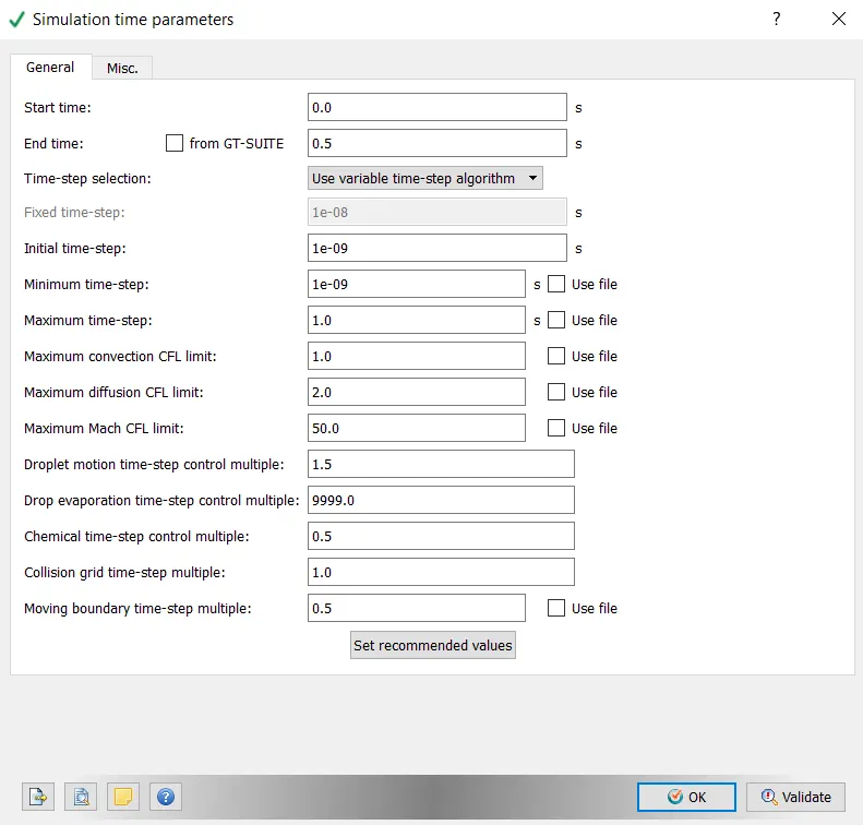
Simulation Time Parameters

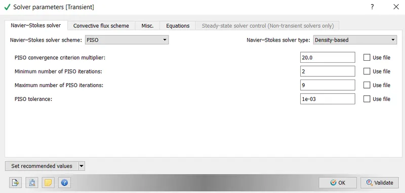
Solver Parameters

Material

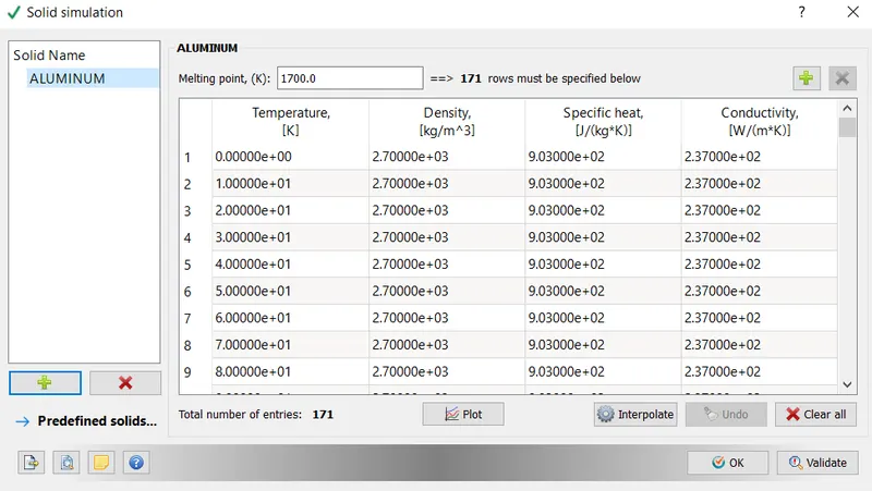
Solid Simulation

Transport properties of gas

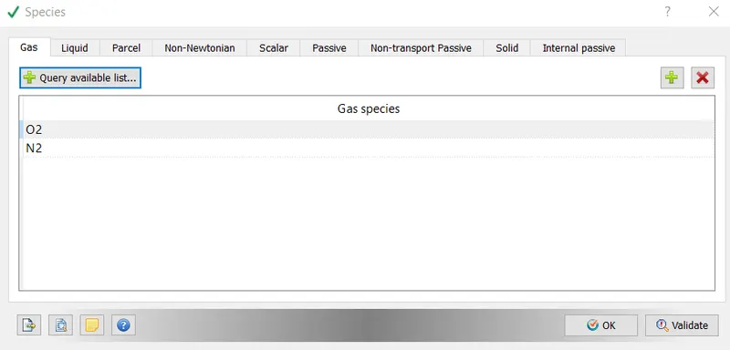
Gas Species

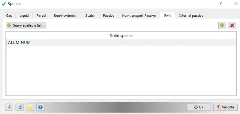
Solid Species

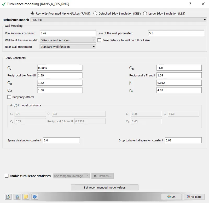
Turbulence Modelling

K - epsilon turbulence model has been used as per default settings.

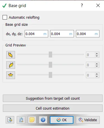
Base grid

The base grid is also as per the case setup.

Super cycling

As discussed super cycling has been set as per case.

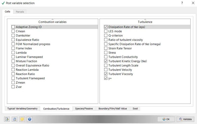
Post Processing variables

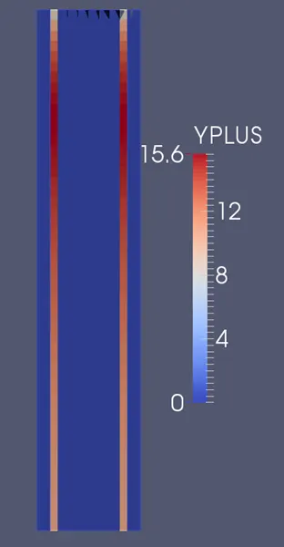
Y+ has been checked in the post processing variables.

Output files

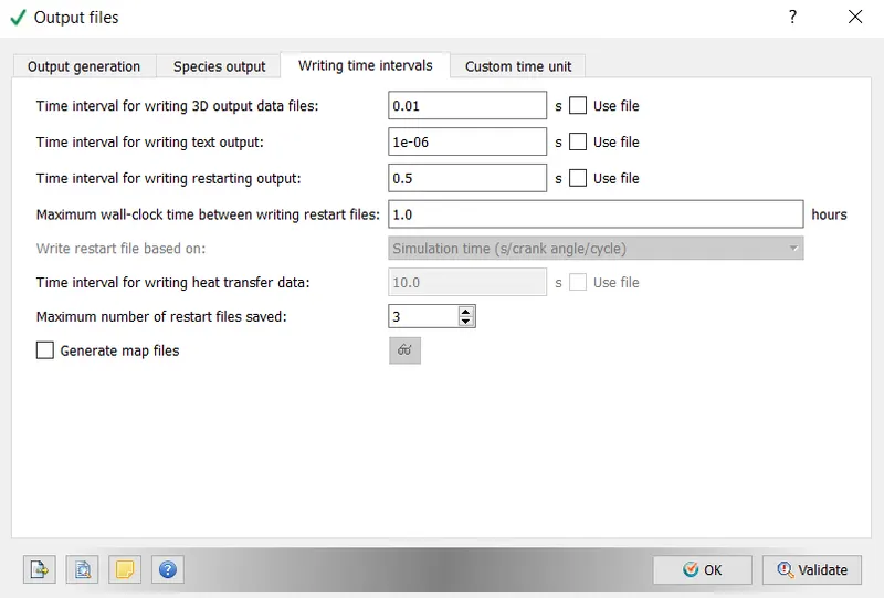
The output has been recorded as per given time steps.

Result and Discussion

Grid Size

Mesh Refinement

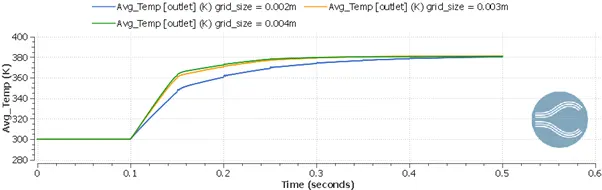
The above plot presents the average temperature calculated at the outlet of the pipe. The value of average temperature at the outlet is assumed to be the control variable for grid independence test. From the plot it is evident that, refining mesh gives little to no change in the control variable. Making the grid size of 0.004m reasonably more efficient as far as utilization of computational resource is concerned.

Grid Size = 0.004m, Super Cycling Interval = 0.05s

Temperature Contour

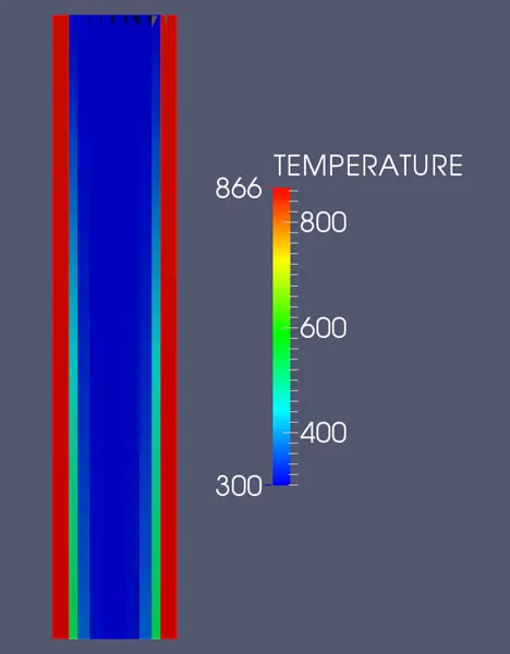
Temperature Animation

Velocity Contour

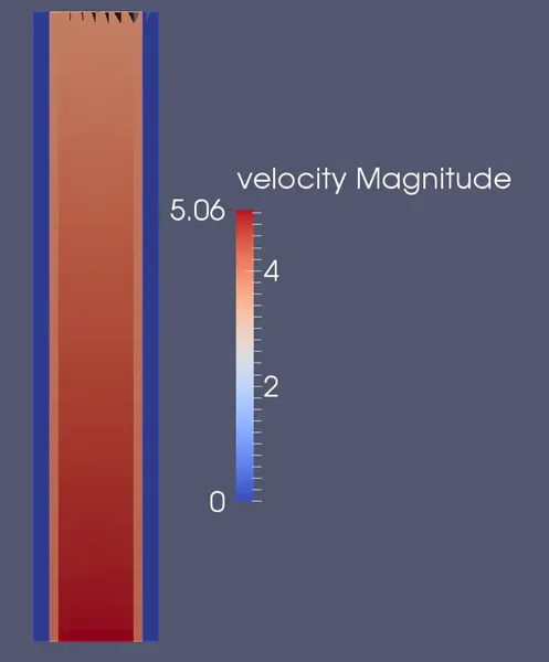
Yplus

Effect of Super Cycling

Conclusions

The grid refinement test was successfully completed and in order for optimizing utilization of computation resource, simulation with maximum grid size is chosen for further study, as there were not significant variation in the results at final time.

Decrease in super cycling interval enables, the results to converge quickly. Since decrease in the interval leads to communication of solution at the interval quicky and more frequently, the solution appears to converge fast as compared to large cycle time.