Conjugate Heat Transfer Simulation

Aim:-

• Setup the CHT simulation flow through the pipe in converge CFD.
• Maintain the inlet Reynolds number as 7000
• Turn on the Y+ value before exporting all the setup files.
• Run grid dependence test by showing outlet temperatures are converging to a particular value.
• Find out the effect of supercycle stage interval by setting supercycle stage interval to 0.01,0.02and0.03.
• Compare the simulation time for the above three supercycle stage intervals.

Objectives:-

• Create the geometry of the pipe with the fluid region.
• Specify the boundary definition to the Geometry.
• Setup Baseline Conjugated heat transfer simulation for the flow through the pipe.
• Calculate the inlet velocity for the Reynolds number and provide the Dirichlet boundary condition for the velocity at the inlet.
• Use the K-Epsilon turbulence model.
• Add Supercycling parameters. Simulate the baseline simulation by using three different Supercycling parameters and observe the simulation time.
• Add additional 3D output Y+ to “post.in” file.
• Simulate the setup with three different mesh grids to perform a mesh dependence test.
• Capture the images of generated mesh from the paraview.
• Finally, generate the animation and upload it on YouTube.

CONJUGATE HEAT TRANSFER ANALYSIS

The Conjugate Heat Transfer (CHT) analysis type allows for the simulation of heat transfer between solid and fluid domains by exchanging thermal energy at the interface between them.

In solids, conduction often dominates whereas, in fluids, convection usually dominates.

Typical applications of this analysis type exist as, but are not limited to, the simulation of heat exchangers, cooling of electronic equipment, and general-purpose cooling and heating systems.

HEAT TRANSFER BY SOLID AND FLUIDS

Heat transfer in a Solid

In most cases, heat transfer in solids, if only due to conduction, is described by Fourier’s law defining the conductive heat flux, q, proportional to the temperature gradient:

`q=-k Delta T`

For time-dependent problem, the temperature field in an immobile solid verifies the following form of the heat equation:

`rho C_p (del T)/(delt) = Delta . (k.DeltaT)+Q`

Heat Transfer in a Fluid

Due to the fluid motion, three contributions to the heat equation are included:

• The transportation of fluid implies energy transport too, which appears in the heat equation as the convective contribution. Depending on the thermal properties of the fluid and on the flow regime, either the convective or the conductive heat transfer can dominate.
• The viscous effect of the fluid flow produces fluid heating. These terms in often neglected, nevertheless, their contribution is noticeable for fast flow in viscous fluids.
• As soon as a fluid density is temperature-dependent, a pressure work term contributes to the heat equation. This accounts for the well-known effect that, for example, compressing air produces heat.

According to these contributions, in addition to conduction, results in the following transient heat equation for the temperature field in a fluid:

`rhoC_p(del T)/(del t) + rho C_p u.del T = alpha_p T ((del p_A)/(del t) + tau . S + Delta . (k Delta T)+Q)`

Geometry Creation:-

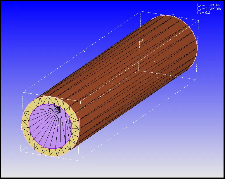
Geometry was created by creating two cylinders. One cylinder, the outer one, is the solid region, and another one, is the fluid region. Some Geometry cleanup operation was performed to avoid interaction between the inner cylinder and the outer cylinder.

Boundary Definition:-

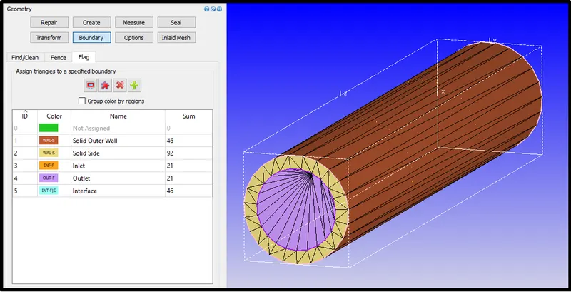
• After geometry creation, the boundary name was assigned to each surface. The outer cylindrical wall was defined as a Solid outer wall. Side solid surfaces of the pipe were defined as solid sides.
• For Fluid surfaces, inlet and outlet surfaces were defined as exhibited in the below figure.
• Now, there is one inner cylindrical surface shared by both fluid and solid, which acts as an interface, so the interface name was given to that particular surface.

Case Setup Parameters For CHT simulation:-

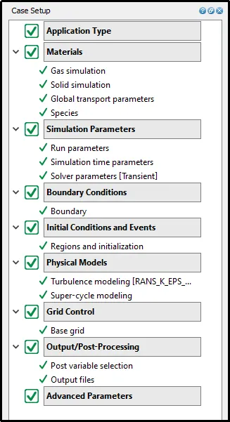
The following parameters were considered while doing the conjugated heat transfer simulation of flow through the pipe.

Simulation Setup/ Case setup:-

Application type:-

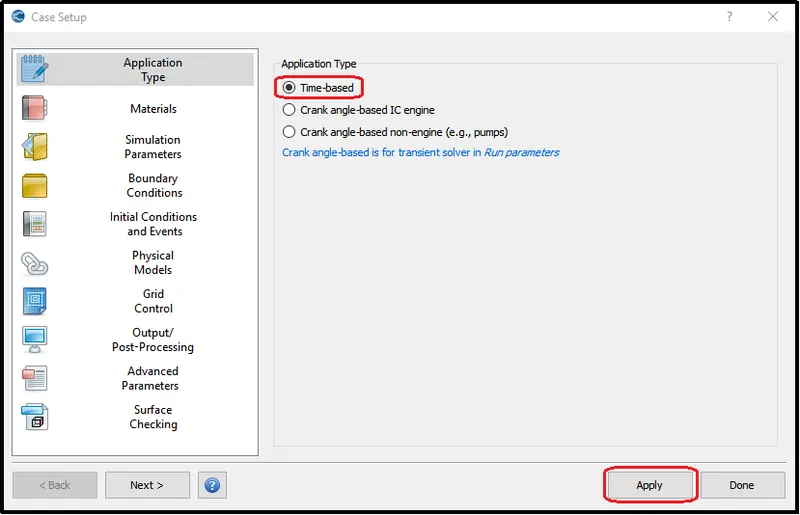
To begin with the transient state simulation in the 'Application Type" the "Time-based" must be selected and then, click apply and done.

Material Definition:-

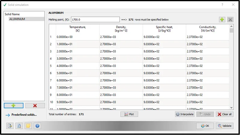
For Solid, Aluminum material was selected from the converge library.

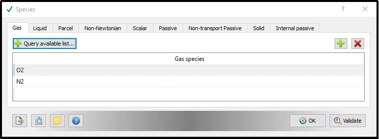
And, for Liquid, Air species - O2 and N2 was defined.

Run Parameters:-

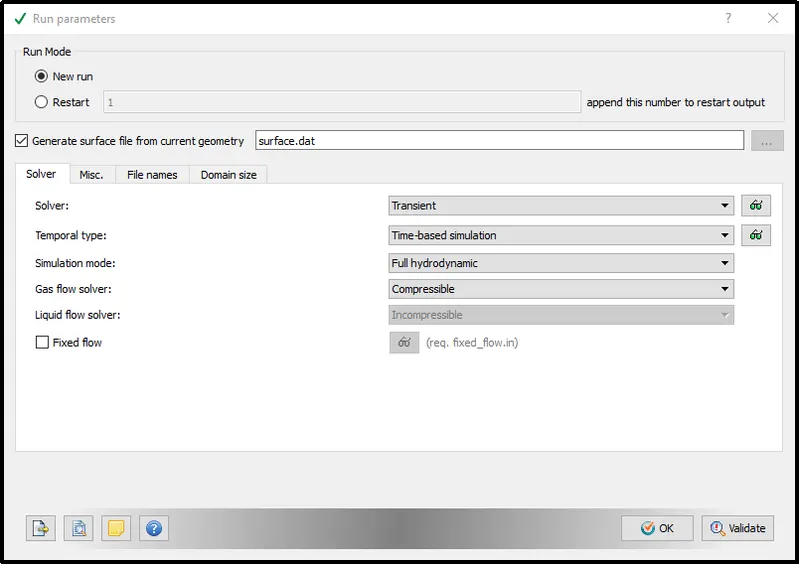
In the run parameter, we get to decide that either, we want steady-state simulation or Transient state simulation, so for the current simulation, the transient solver type was selected.

And, finally, as we are using air as a fluid that is compressible in nature so gas flow solver is set as compressible.

Simulation time parameters:-

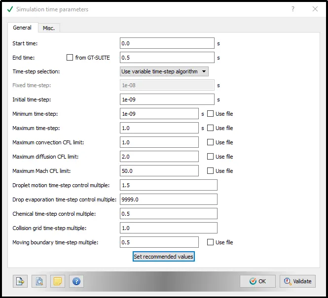
For the transient simulation, we have to set the run time of the simulation. So for the run time calculation, we require the flow length and velocity.

`R u n T i m e = (F l o w L e n g h t) /(V e l o c i t y)`

From the pipe geometry, the maximum Flow length is 0.2m

`R u n T i m e = 0.2/8`

`R u n T i m e = 0.025 sec`

Suppose we are going to simulate 20 times airflow from inlet to outlet.

Then, `R u n T i m e = 0.025xx20`

Therefore, `R u n T i m e = 0.5 sec`

Fluid And Solid Region:-

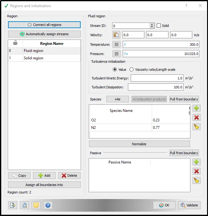
This particular simulation involves both fluid and solids, so the two separate regions were created.

For the liquid region following initial parameters were considered. and Stream ID set to 0.

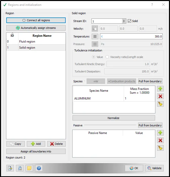
Whereas, for Solids, the stream ID was set to 1. Aluminum material was mentioned.

• A Stream is a collection of connection regions of the same phase(fluid, said, etc)
• CONVERGE solves for each stream independently except for the coupled interfaces.
• CONVERGE creates the mesh for each stream Independently and this allows for different embedding levels on either side of the interface.

Boundary Conditions:-

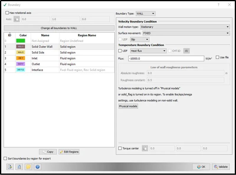
Solid Outer Wall:-

The outer cylindrical face is the part of the solid region so define it as a solid region.

At the solid outer wall, we are considering the Newman boundary condition where you prescribe a flux, which is the gradient of the dependent variable.

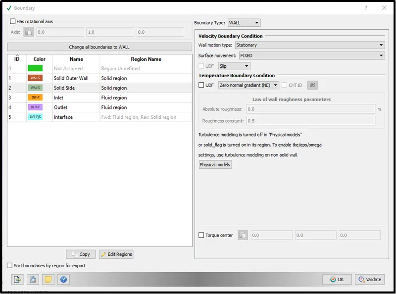
Solid Side near Inlet and Outlet

Here, a zero normal gradient case is considered for temperature.

Inlet:-

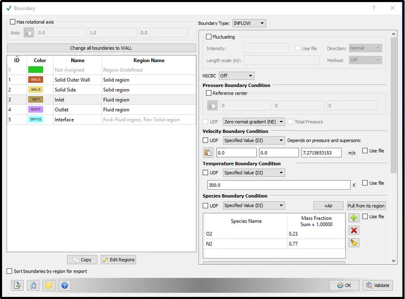
Near the inlet, the velocity was calculated to maintain the specific Reynolds number as 7000.

`Re = (rhoxxVxxD)/(Dynamic Visc o sity)`

`V=(Rexxmu)/(rhoxxD)`

`V=(7000xx1.849xx10^-5)/(1.184xx0.015)=7.28772522523 m//s`

We are considering the inlet boundary condition as a Dirichlet boundary condition by specifying all the inlet values of velocity and temperature.

Outlet:-

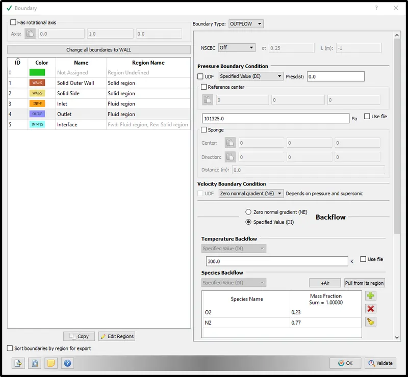
For the outlet, also considering the inlet boundary condition as a Dirichlet boundary condition by specifying all the inlet values of pressure, and temperature.

Fluid-Solid Interface:-

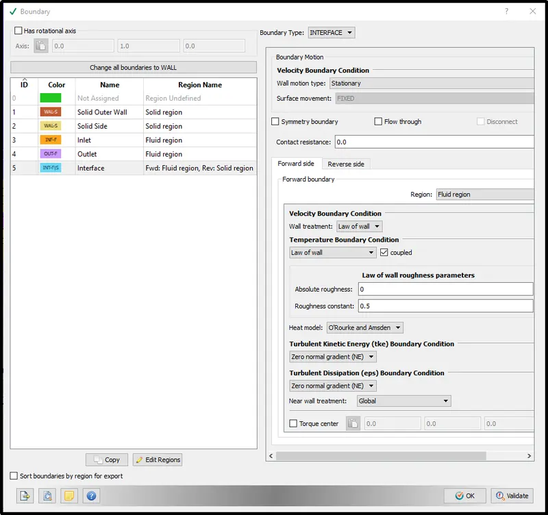
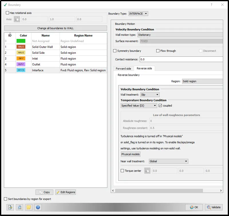
• Interface boundary separates the two types of material or phases. CHT simulation requires at least one Interface boundary.
• we must define boundary conditions for the forward and reverse boundary of each INTERFACE.
• Ensure that the normal vectors are correct to the specific forward/ reverse direction.

Fluid Interface:-

Solid Interface:-

Turbulence model:-

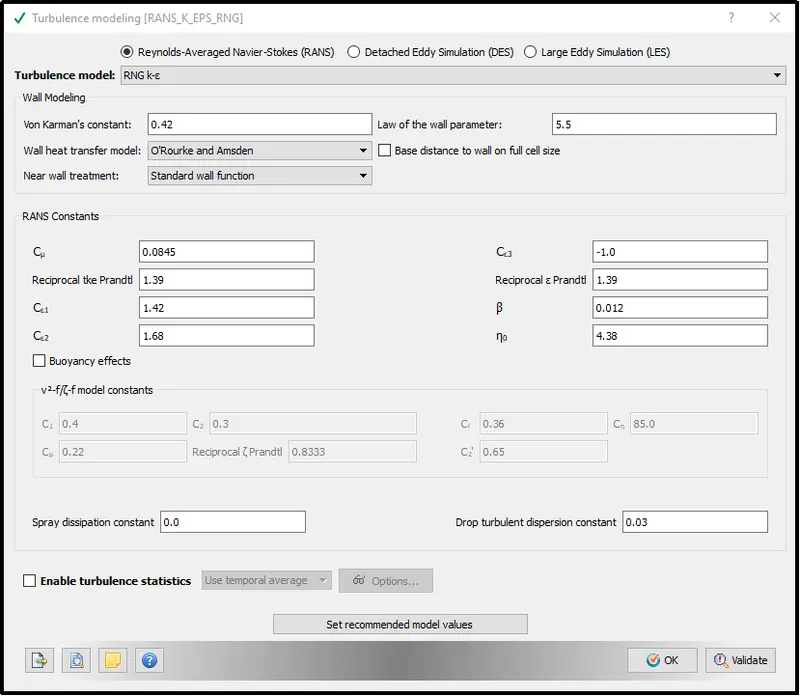
Here, the turbulence model was used as RNG K-epsilon. because because of obstacle or throttle valve the laminar stream converted into turbulent.

Super-Cycle Modeling:-

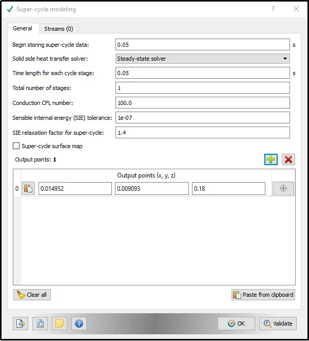
In super-cycling CONVERGE iterates between fully-coupled transient and steady-state solution methods for the solid only. (CONVERGE uses the transient solver for the fluid)

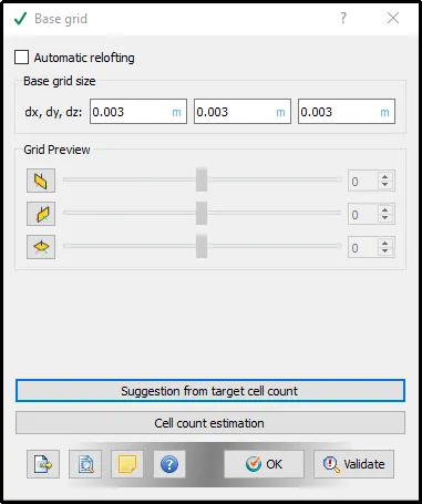
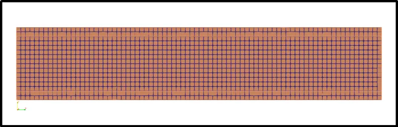
Base Grid Definition:-

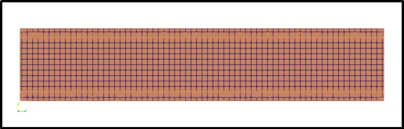
Result of Above Base grid:-

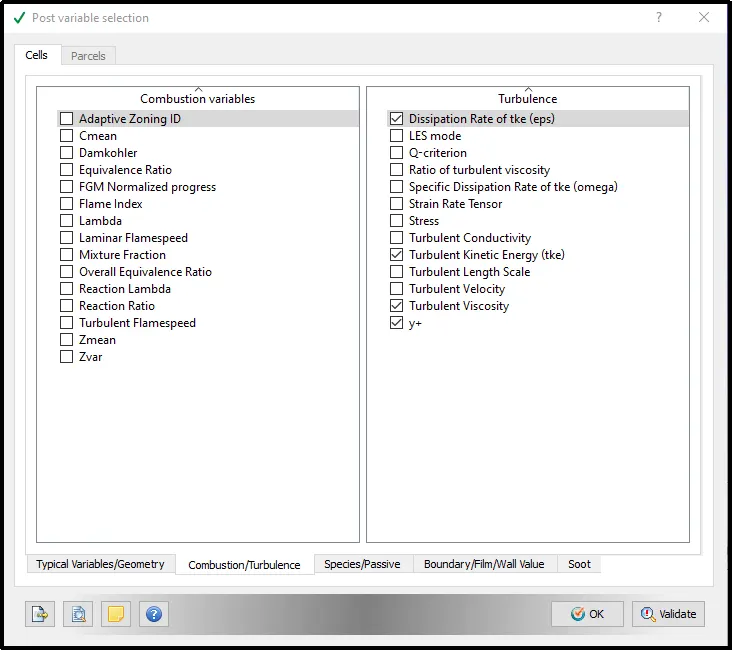
Post variable selection:-

Check the Y+ option to add it to the post.in the file as additional 3D outputs.

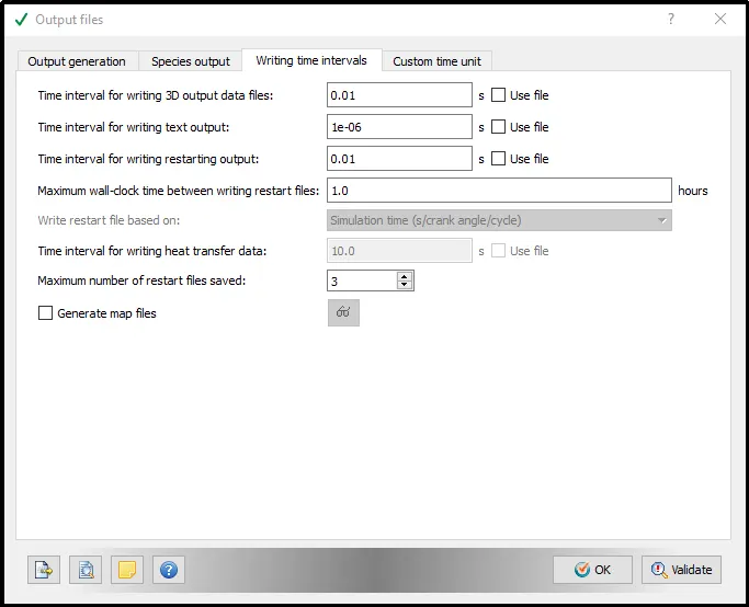
Output Files setting:-

Results:-

Simulation Case 1:-

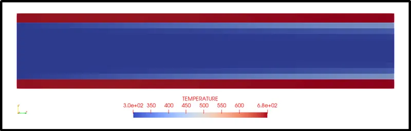
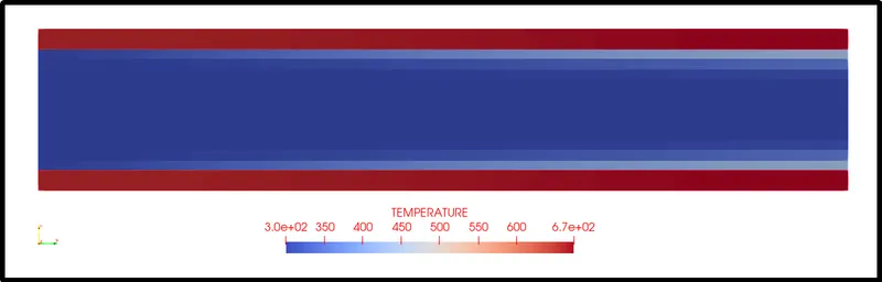
Temperature Contour:-

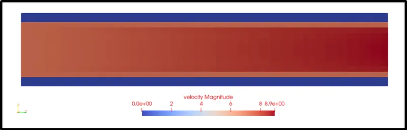
Velocity Contour:-

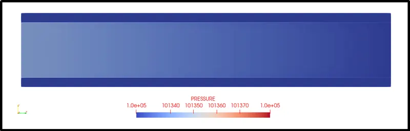
Pressure Contour:-

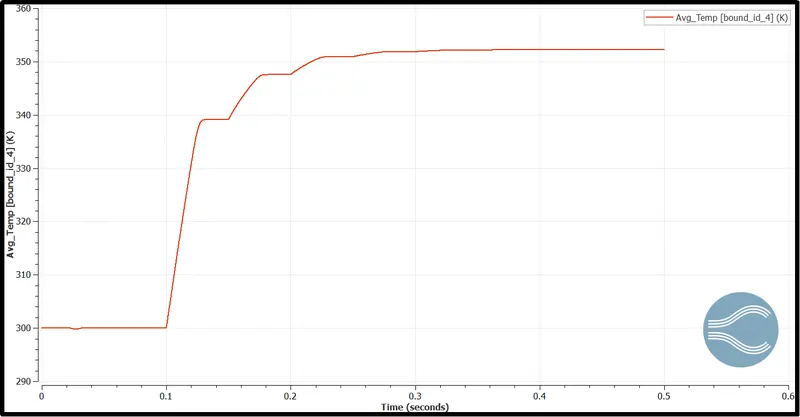
Average Temperature at Outlet:-

Simulation Case 2:-

Temperature Contour:-

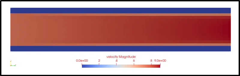
Velocity Contour:-

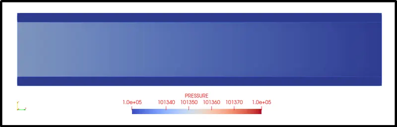
Pressure Contour:-

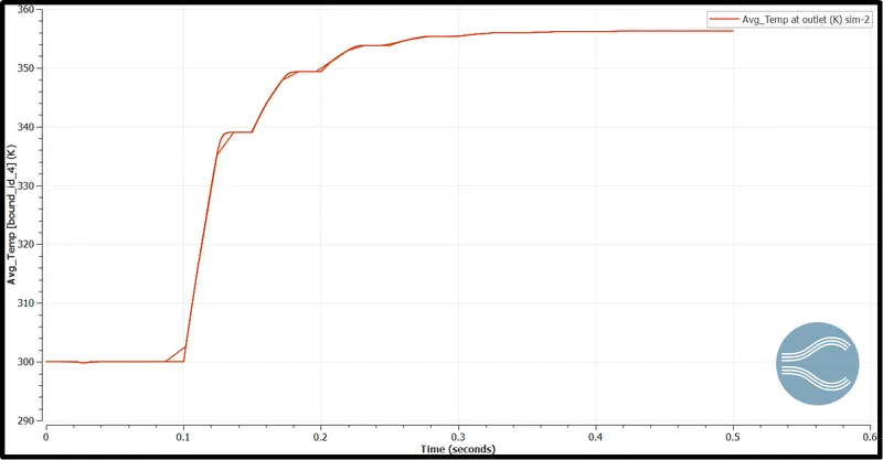
Average Temperature at Outlet:-

Simulation Case 3:-

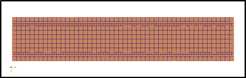
Fixed embedding was used for this case.

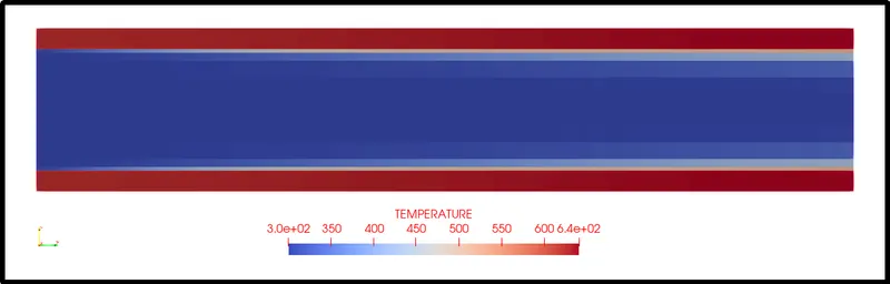
Temperature Contour:-

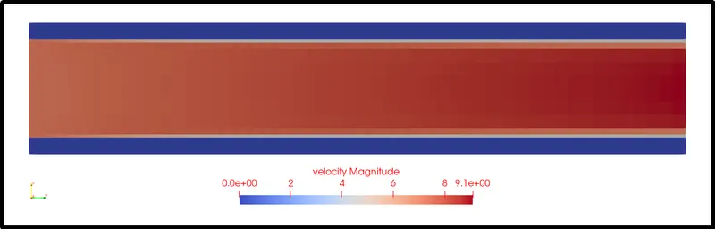
Velocity Contour:-

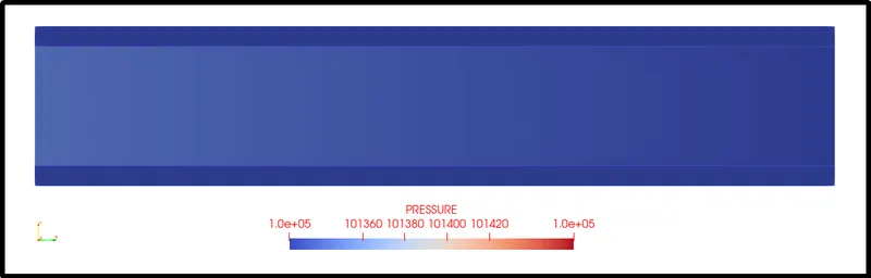
Pressure Contour:-

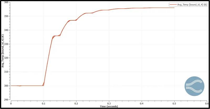
Average Temperature at Outlet:-

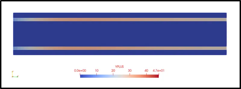
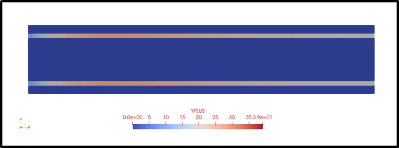
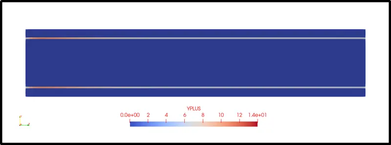
Y+ Value:-

Y+ Boundary layer

The behavior of the flow near the wall is a complicated phenomenon and to distinguish the different regions near the wall the concept of wall Y+ has been formulated. Thus Y+ is a dimensionless quantity and is the distance from the wall measure in terms of viscous length.

In the turbulent boundary layer region flow near the wall has been analyzed in terms of three layers.

• The inner layer, or sublayer, where viscous shear dominates.
• The outer layer, or defect layer, where large-scale turbulence eddy shear dominates.
• The overlapping layer, or log layer where velocity profiles exhibit a logarithmic variation

One of the reasons for the need for Y+ is to distinguish different regions near the wall or in the viscous region, however, how exactly it helps in turbulence modeling or general CFD modeling needs to be well understood. If we intend to resolve the effects near the wall i.e., in the viscous sublayer then the size of the mesh size should be small and dense enough near the wall so that almost all the effects are captured. But in some cases, if the wall effects are negligible then there is the option of including semi-empirical formulae to bridge between the viscosity-affected region and fully turbulent region, and in this case, the mesh need not be dense or small near the wall i.e, the coarse mesh would work.

For Simulation Case1:-

For Simulation Case2:-

For Simulation Case3:-

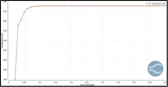
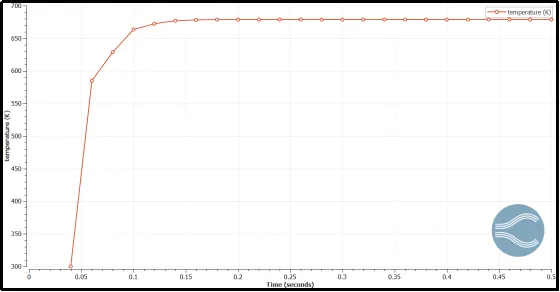
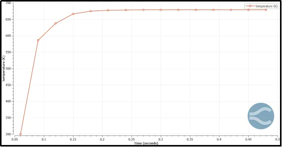
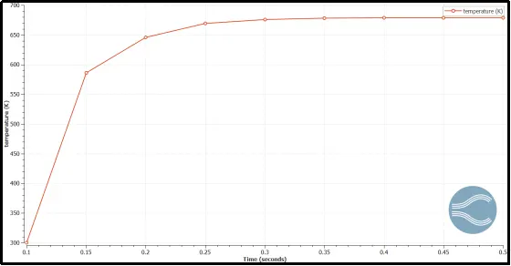
Temperature Vs Time of the solid with the variation of Supercycle Stage Interval

• During super-cycling CONVERGE solves the fluid and the solid together with the transient solver and stores the instantaneous heat transfer coefficients and temperatures on the interface during this process.
• Then it freezes the fluid solver and time average the heat transfer coefficients and temperatures and applies them as the boundary conditions at the interface.
• Afterward, solves the solid temperature until it reaches a steady-state. then it updates the solid temperature field and unfreezes the fluid solver.
• CONVERGE repeats this process until the solid temperature converges.

Supercycle Stage Interval 0.01:-

Supercycle Stage Interval 0.02:-

Supercycle Stage Interval 0.03:-

Supercycle Stage Interval 0.05:-

Observation Table1:-

With all the grid sizes we are getting the almost same results, which means the setup is correct and simulation results are dependable. Thus, results pass the grid independence test.

Observation Table2:-

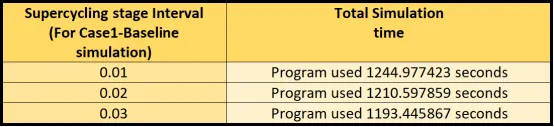
By observation table2, we can notice, by reducing the supercycle stage interval our simulation time increases.

Temperaure Variation Animation:-

Conclusion:-

• Heat transfer coefficient is the function of properties of the fluid at film temperature, temperature difference, temperature coefficient, buoyance force, etc., hence, mesh resolution near the walls usually has the biggest impact on numerical results.
• simulating the results with different grid sizes is very important to check the mesh independence test.
• Fixed embedding is a great tool to refine mesh near the required surfaces of the parts.
• In super-cycling CONVERGE iterates between fully-coupled transient and steady-state solution methods for the solid only. (CONVERGE uses the transient solver for the fluid)
• As we lower the supercycle stage interval simulation time of setup rises.

References:-

[1] Conjugated Heat Transfer - https://www.comsol.com/blogs/conjugate-heat-transfer/

[2] Effect of thermal boundary condition on forced convection from circular cylinders - https://www.researchgate.net/publication/334660107_Effect_of_thermal_boundary_condition_on_forced_convection_from_circular_cylinders

[3] Heat transfer coefficient - https://en.wikipedia.org/wiki/Heat_transfer_coefficient