Week 6: Conjugate Heat Transfer Simulation

1. Title – Conjugate Heat Transfer Simulation.

2. Objective –

• To create the hollow cylinder in converge Software.
• To set up the case with proper grid size, material and boundary conditions.
• To solve the case using Cygwin terminal and convert the result for Paraview software.
• To import output files in Paraview and generate required contours and plots.

3. Theory –

Conjugate heat transfer (CHT) – this is analysis which allows the heat transfer between fluid and solid by energy interaction. CHT analysis can accurately predict heat transfer by simultaneous solving all the relevant solid and flow field heat transfer processes. CHT analysis predicts heat transfer properties where heat interaction is between solid body and fluid. CHT has many applications like simulation of cooling of electronic component, simulation of heat exchangers. In the real-world phenomenon mostly three modes of heat transfer acts together, that why it is necessary to study CHT.

In this study we will see heat interaction between aluminium cylinder and air. We will perform grid independency test also to find out the effect of mesh on temperature.

4. Procedure –

Geometry -

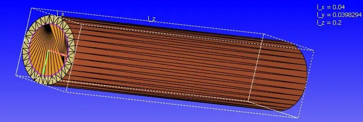
In this study we performed CHT analysis with three different supercycle stage interval, for that the following procedure was followed –

1. Starting with application type, which is time based, since it is not related to IC engine applications.

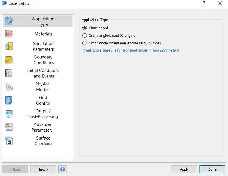
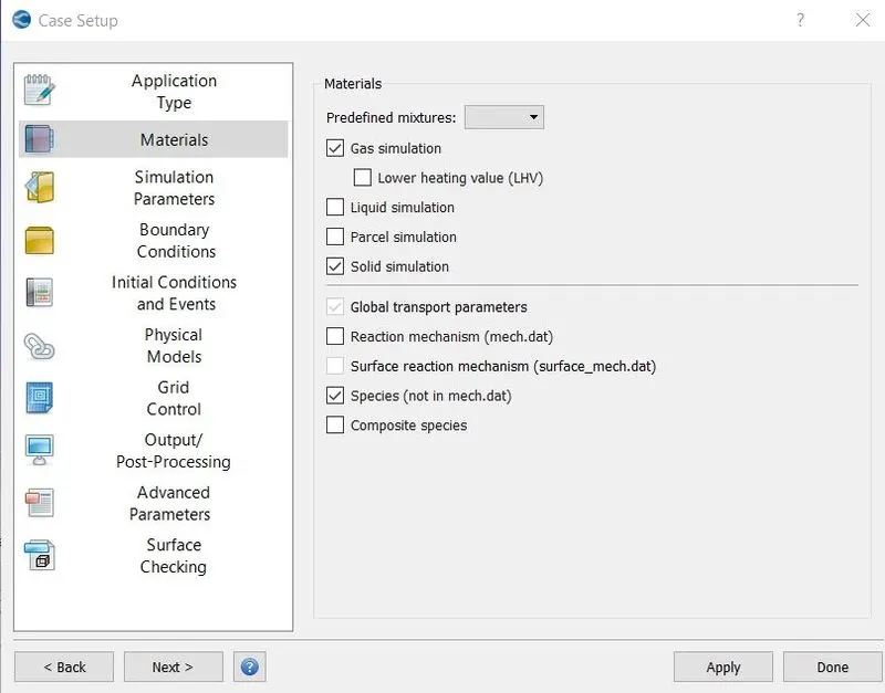
2. Air chosen as fluid material and reaction mechanism was disabled. Solid simulation was enabled. In solid simulation menu aluminium was selected, this was responsible for the heat transfer to air. Species was also enabled, to define which species are taking part in simulation.

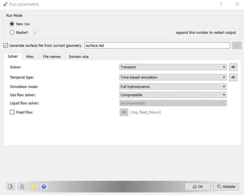
3. In run parameters transient solver chosen as solver type, simulation mode was chosen as full hydrodynamic because we want to simulate with effects of fluid also.

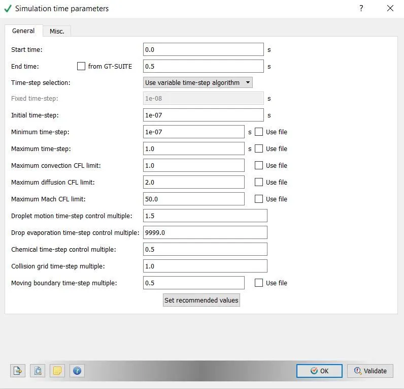
4. In simulation time parameter start time 0s, end time 0.5s, initial time step 1e-07s, minimum time step 1e-07s, maximum time step 1s was chosen.

5. In solver parameters pressure-based solver was chosen, other parameters kept unchanged.

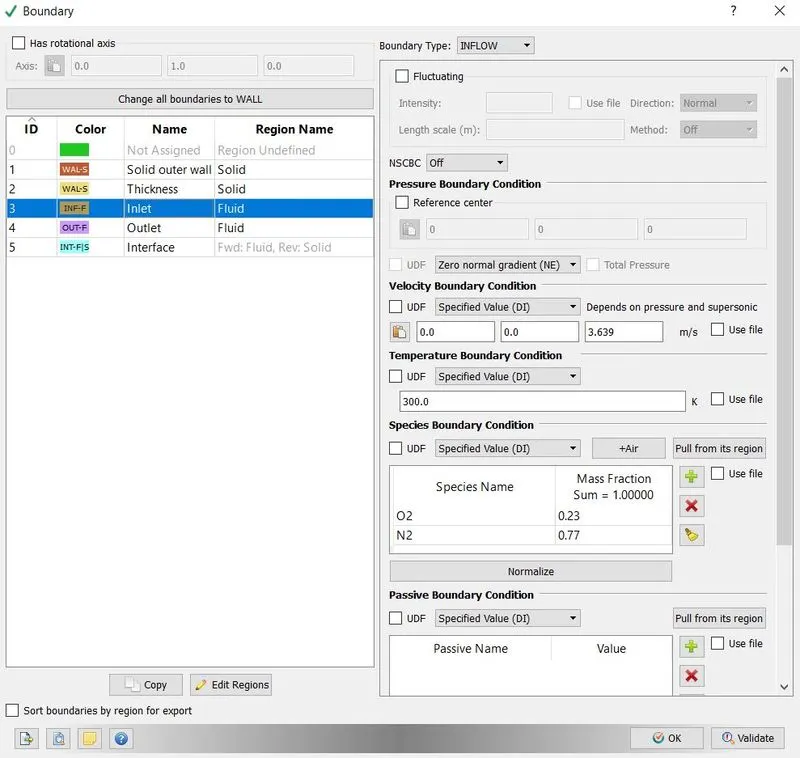
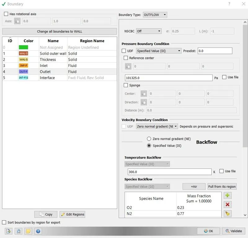
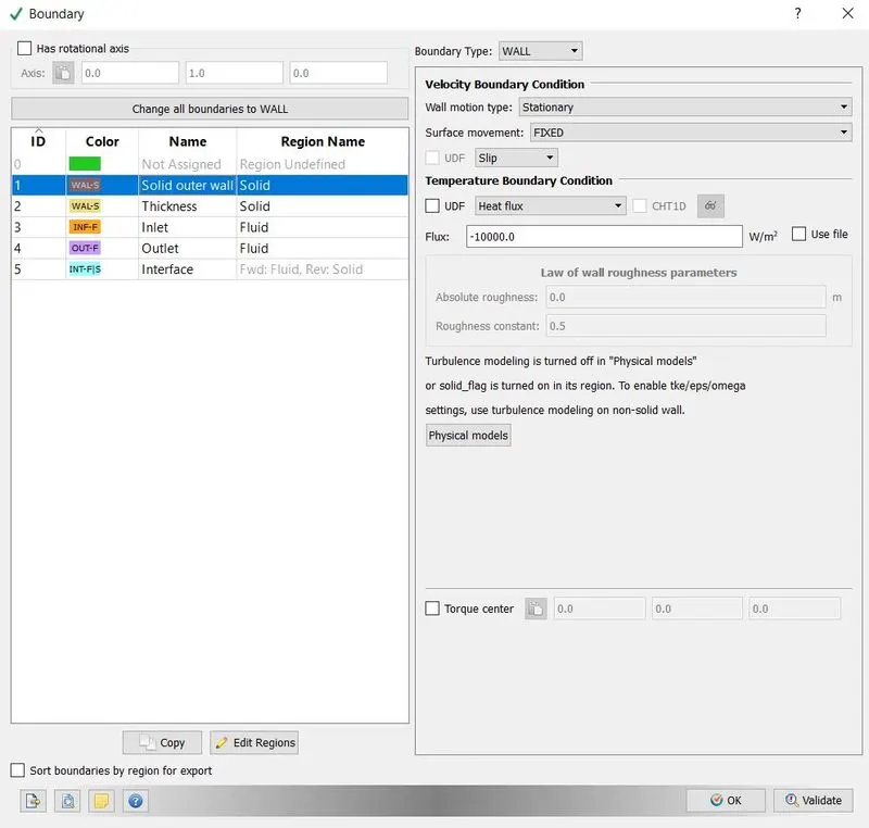
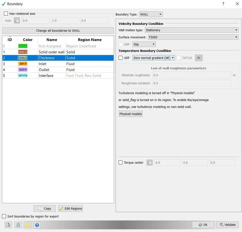
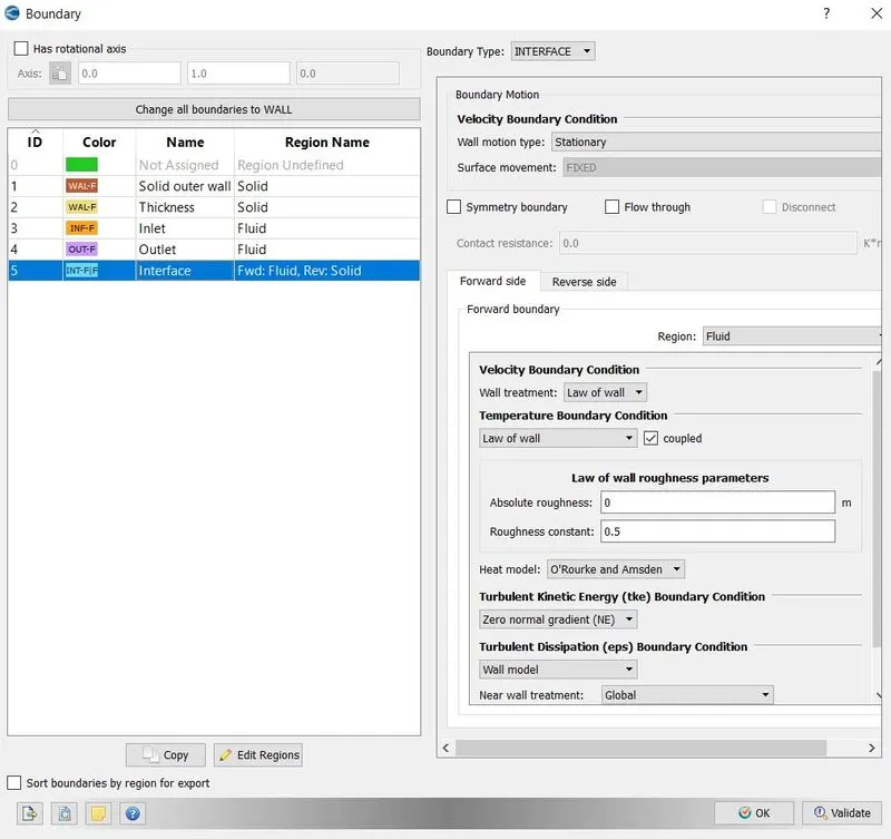
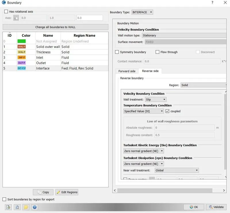
6. In boundary conditions solid outer wall, thickness, inlet, outlet and interface was defined. Solid outer wall was set with heat flux -10000 W/m^2, we gave negative value because heat is leaving the wall. Thickness was treated as wall with no temperature values, at inlet boundary we gave velocity 3.639m/s, which is calculated to maintain Reynolds number 7000. At outlet pressure value was set 101325pa. at interface parameters of solid and fluid was defined as shown following image.The velocity calculation was done by following formula -

Reynolds Number = density of fluid*velocity of fluid*characteristic length/dynamic viscosity

Reynolds number -7000

Density of fluid – 1.184 Kg/m^3

Velocity of fluid – v

Characteristic length –0.0398m

Dynamic viscosity -1.849*10^-5 Kg/ms

7000 = 1.184*v*0.0398/1.849*10^-5

v = 3.639 m/s

Boundary conditions -

Inlet -

Outlet -

Solid wall -

Thickness -

Interface -

7. We went with default turbulence model which was Reynolds Averaged Navier Stokes k-epsilon model.

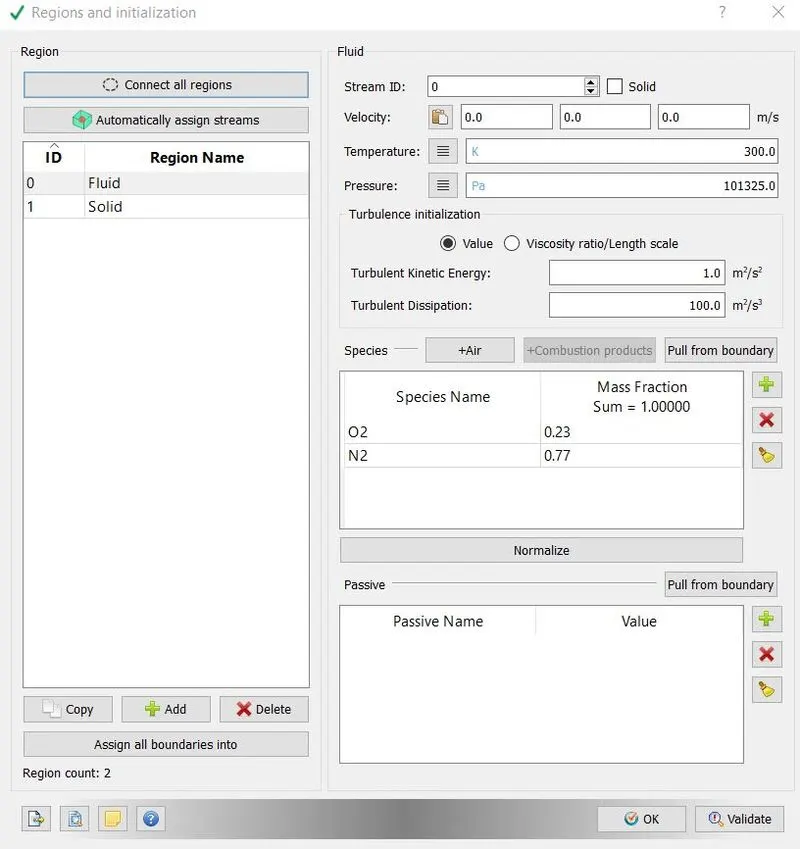
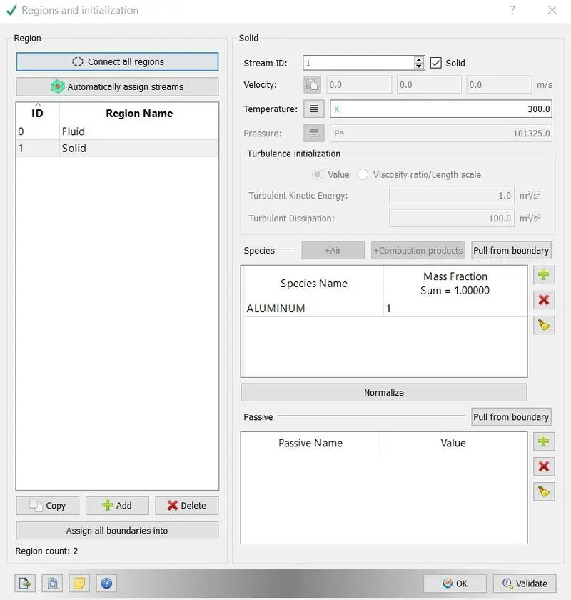
8. In this simulation we had two regions solid and fluid, so these we defined in regions and initialization menu with their parameter. After this, boundaries were set to the region, inlet and outlet was set to fluid and others to solid.

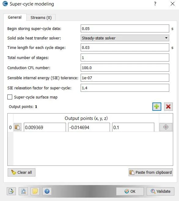
9. In physical model Super-cycling option was enabled. This is unique concept of converge software, which is used to solved CHT problems. Solid and fluid solver can not be solved together because, fluid solver reaches steady state faster than solid one, due to time scale difference. Super cycling concept pauses fluid solver until solid reaches steady state. Time interval is defined by user.in this simulation we altered only two parameters and other were same. Begin storin super cycle data is the time where super cycle starts to store data were set it with 0.05s, it should be equal or less than simulation time. Time scale for each cycle stage is the where fluid solver paused and solid solver finds converged values. We set it with three different values 0.03,0.02,0.01, because we wanted to study the effect of this parameter on temperature.

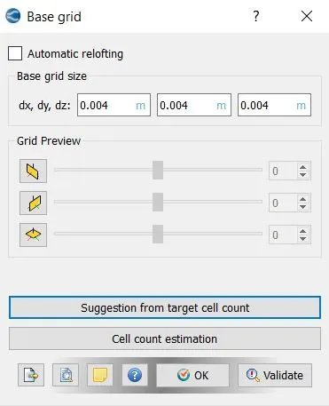
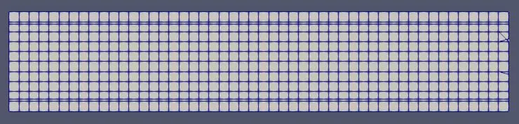
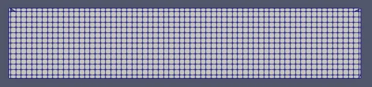
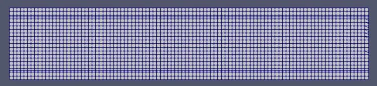
10. We used three different grids with sizes 0.002m,0.003m0.004m, which was given in base grid parameter.

11. Post variable selection allows us to select variables which we want to analyse in post processor. Converge has some variables as defaults, but addition to that y plus was selected from turbulence menu.

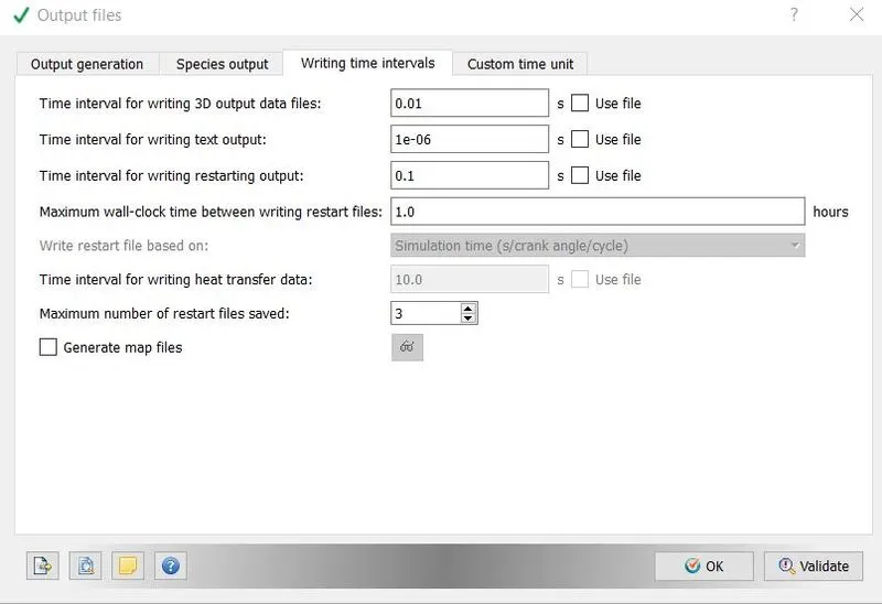
12. In output files 0.01s was given as time interval to write 3D outputs, 0.1 for restarting output and 1e-06s for writing text output.

13. Input files exported in a folder and these solved using Cygwin terminal.

14. Files were converted into converge 3D postprocessing option and postprocessed in Paraview.

5. Results -

Case1

Grid size 0.004

Mesh -

Temperature Contour -

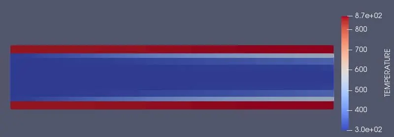
Temperature animation -

https://drive.google.com/file/d/1gdfj2Mc0-nL6XyMduJRpA5QX4kaq8H0L/view?usp=sharing

Grid size 0.003

Mesh -

Temperature Contour -

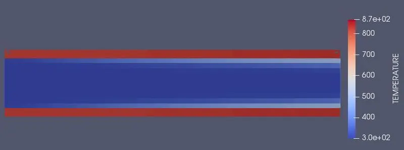
Temperature animation -

https://drive.google.com/file/d/1Kko3_ICjUHROggBc-zCuwKM16YR_DLnz/view?usp=sharing

Grid size 0.002

Mesh -

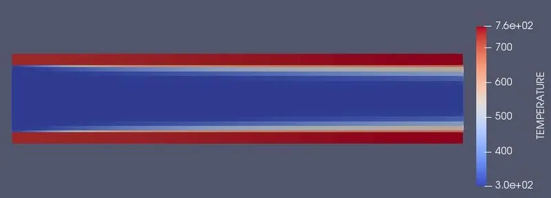
Temperature Contour -

Temperature animation -

https://drive.google.com/file/d/1rHY03VVwr8qjIS8Ucf-TjBOl-XlFGnBc/view?usp=sharing

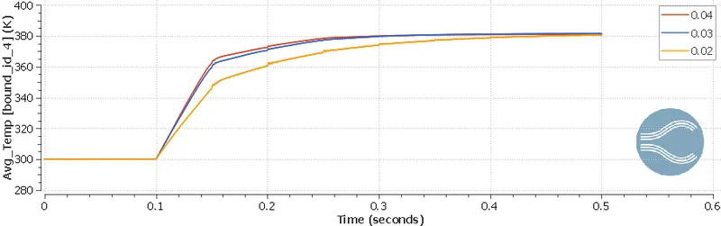
Temperature Plot -

Case2 with Grid size 0.004

Super cycle stage interval 0.03

Temperature contour -

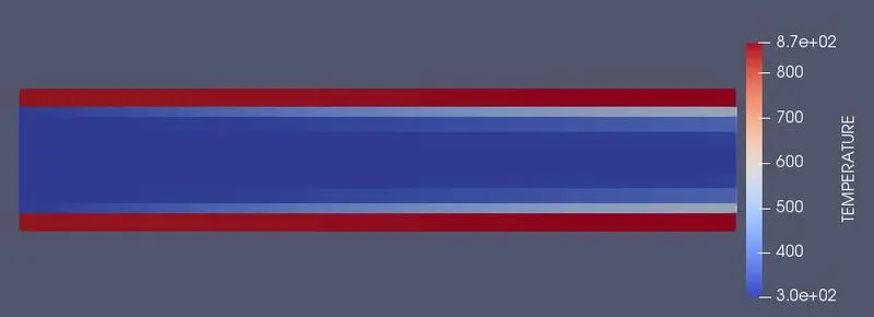
Super cycle stage interval 0.02

Temperature contour -

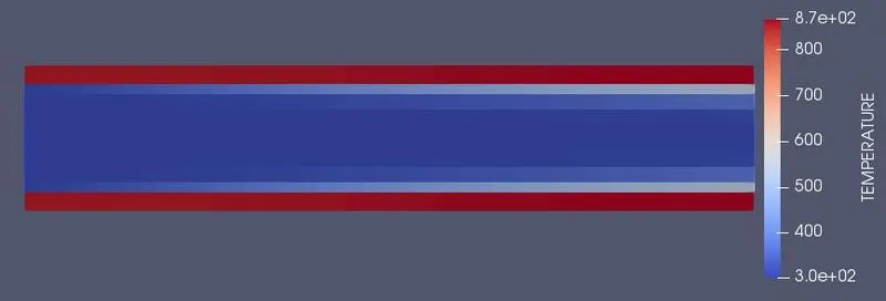
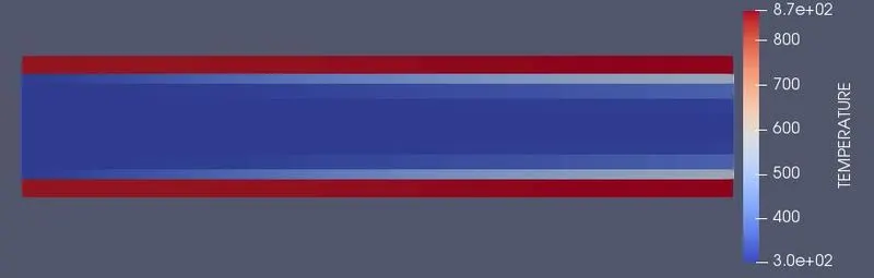
Super cycle stage interval 0.01

Temperature contour -

Temperature Plot -

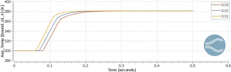
For this simulation there were two aim, first, to see the effect of mesh size on temperature, which is known as mesh independency test and second was to study the effect of super cycling parameter on the temperature. The animations and temperature were created to see how heat is propagating from solid to fluid. We used three different meshes with constant super cycling parameter and a temperature plot was created. We can infer from the plot that temperature values are independent of mesh because for all three different mesh, they are conversing at a particular value of temperature. In second we varied the value of time length for each cycle stage. From the temperature plot of this case, we can say time length parameter of super cycle is disturbing the temperature, at initial time steps only and they are converging to a particular value after some time which 380K, although this is varying after decimal point but that is tolerable. Decrement in time length leads solution to converged faster. If we compare case two with case one, we can say solution converges faster, for a particular value of mesh, here 0.004m was used. In case 1 we got stable temperature 380K at 0.45 but in case two we got at 0.45.