Week 6: Conjugate Heat Transfer Simulation
#Aim:1.To perform Conjugate Heat Transfer Simulation through a circular pipe using Converge studio and Post process with Paraview.
2.Perform Grid dependence test.
3.Study Effect of supercycle stage interval on Simualtion time.
#Introduction:
Conjugate heat transfer, which is the ultimate goal in this work, is a coupled problem involving heat transfer in a fluid domain as well as in the surrounding solid wall. Heat transfer by conduction and convection simultaneously occurs in the majority of engineering applications, such as heat exchangers and fins. Efficiently combining heat transfer in solids and fluids is the key to design effective coolers, heaters, or heat exchangers.
Modelling and design of such heat transfer devices is complicated due to coupling, which involves a rather large number of parameters describing both fluid and solid domains.
#Transient simulation setup using given condition:
Inlet Reynolds number =7000
rho=1.176(@27 degrees)
D=0.015 metre
Dynamic viscocity=1.85*10^-5
since,
Re = (rho*V*D)/(Dynamic viscosity)
rho=Density,
V=Inlet velocity
D=Characterstic Length
V=Re*(Dynamic viscosity)/(rho*D) (m/sec)
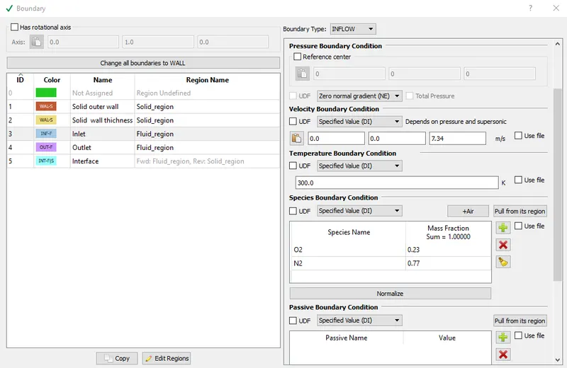
V=7.34 m/sec.
-----------------------------------------------*****************---------------------------------------------
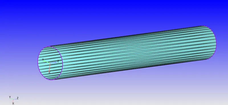
#Geometry :
#Inner cylinder:
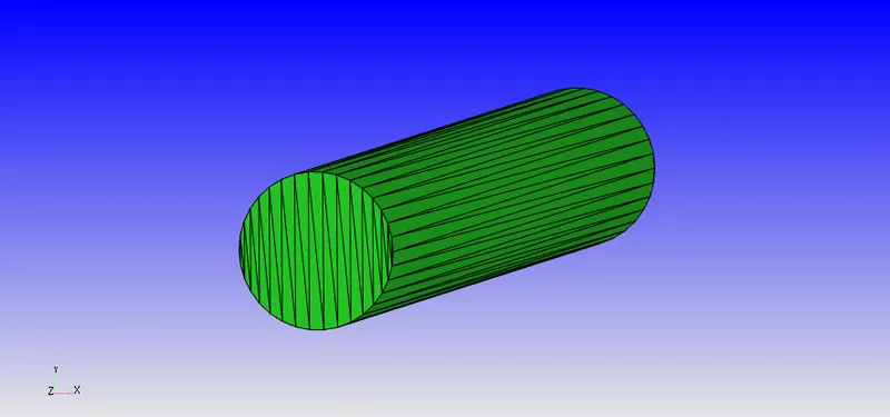
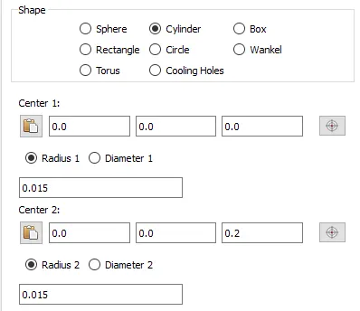
#Outer cylinder:
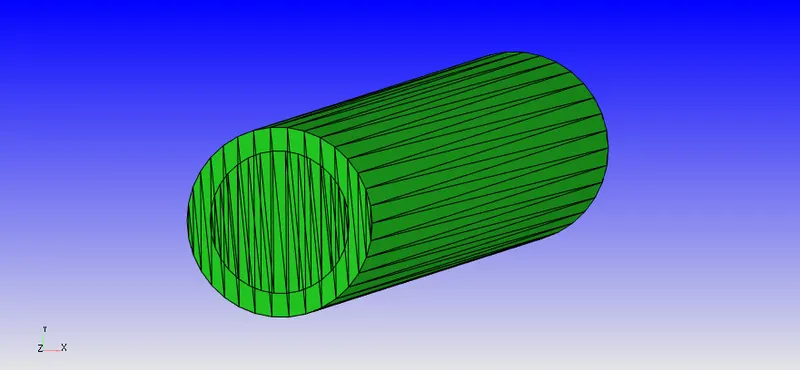
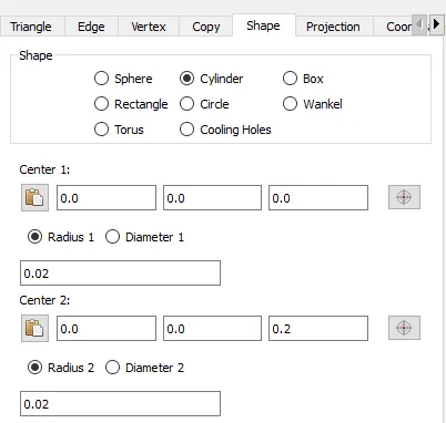
#Flagged geometry:
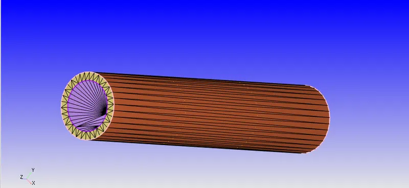
#Solid outer wall:
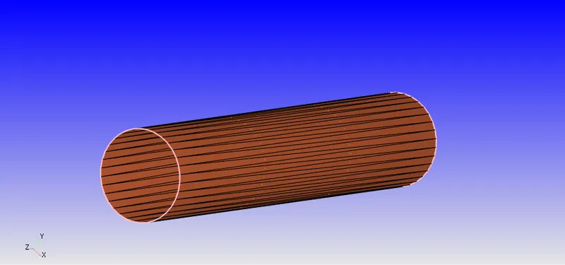
#Solid wall thickness:
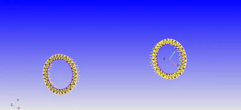
#Inlet and Outlet:
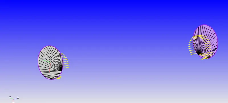
#Interface between solid and fluid region:
--------------------------------------------*************---------------------------------------------------
#Case setup:
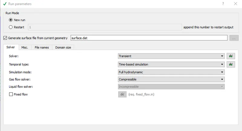
1.Application type-Time based.
2.Materials:-->>Select-->> Gas ,Solid Simulation and species.
Gas simulation-Air (default setting)
Solid simulation-Aluminium
Global transport properties-Default
Species- Gas-N2,O2 ---- Solid-Aluminium
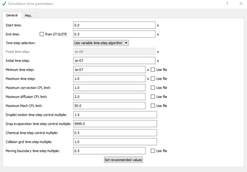
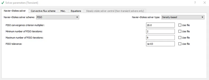
3.Simulation Parameters:
4.Boundary Condition:
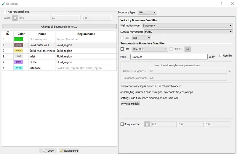
a.Solid Outer wall:Heat flux added-->>>-10000 `W/m^2`
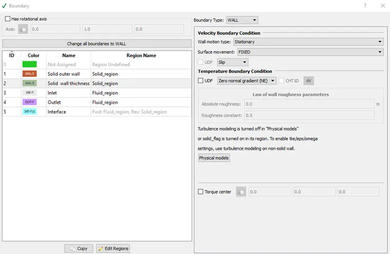
b.Solid wall thickness:
c.Inlet:
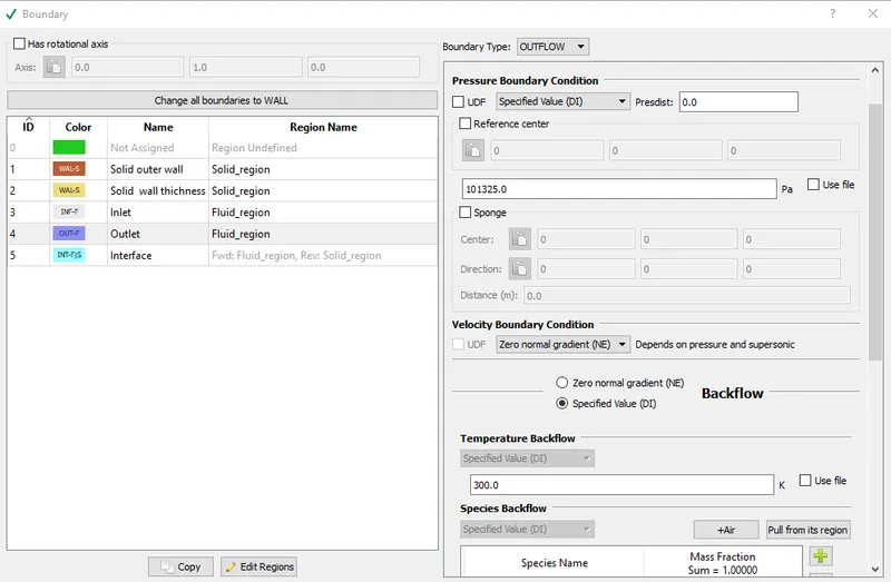
d.Outlet:
e.Interface:
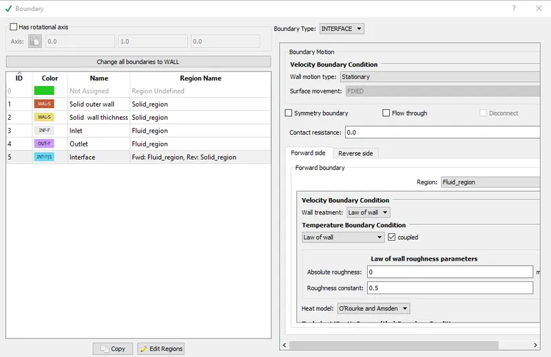
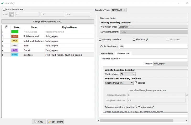
5.Initial conditions and events:
#Regions and initialization:
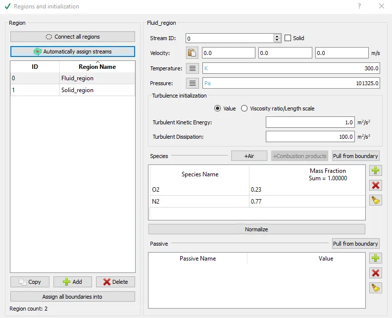
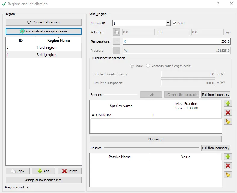
6.Physical Models:
#Turbulence Model-RNG K-epsilon
7.Output and Post process variables:
Add y plus parameter in post variable selection to default setting.
Different Cases that will be discussed:
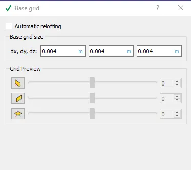
Case-1-->>Grid size-4 mm and Super cycling stage interval--0.05
Case-2-->>Grid size-5 mm and Super cycling stage interval--0.05
Case-3-->>Grid size-6 mm and Super cycling stage interval--0.05
Case-4-->>Grid size-4 mm and Super cycling stage interval--0.01
Case-5-->>Grid size-4 mm and Super cycling stage interval--0.02
Case-6-->>Grid size-4 mm and Super cycling stage interval--0.03
Case-1:-->>Grid size-4 mm and Super cycling stage interval--0.05
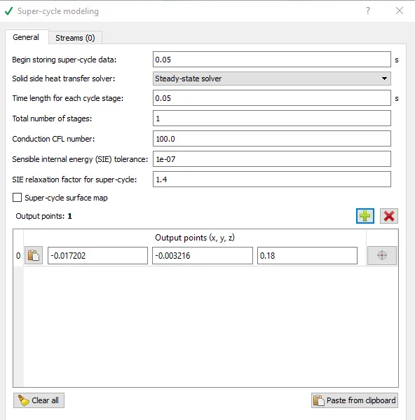
Set super cycling interval-0.05
Create point near Outlet to measure Temperature.
#Results:
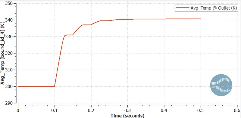
1.Average Temperature @ Outlet line plot:
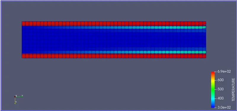
2.Temperature contour plot:
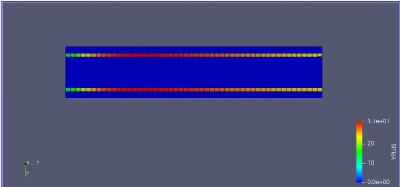
3.Y plus contour plot:
4.Mesh: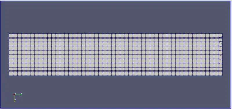
#Link for clip showing rise in fluid temperature due to heat transfer.
---------------------------------------*********************************-----------------------------
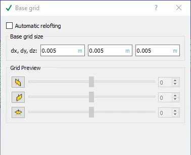
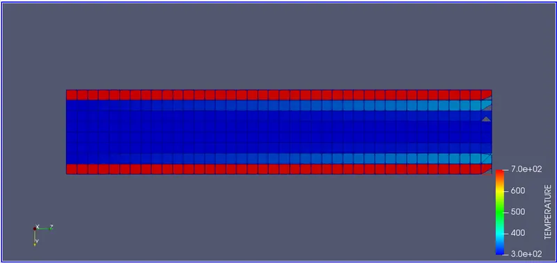
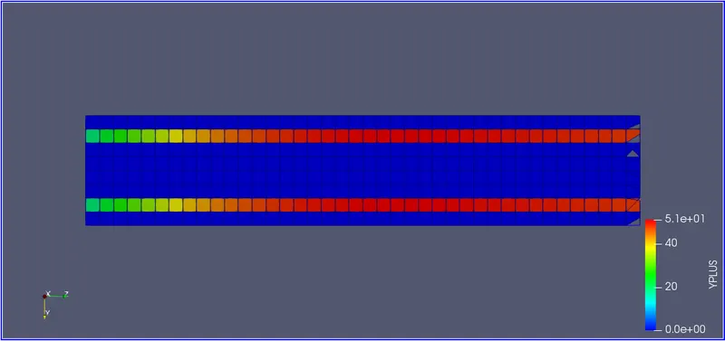
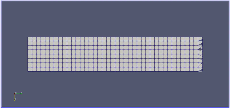
Case-2-->>Grid size-5 mm and Super cycling stage interval--0.05.
#Results:
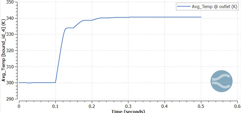
1.Average Temperature @ Outlet line plot:
2.Temperature contour plot:
3.Y plus contour plot:
4.Mesh:
----------------------------------------------****************---------------------------------------------
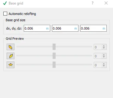
Case-3-->>Grid size-6 mm and Super cycling stage interval--0.05
#Results:
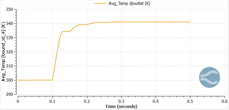
1.Average Temperature @ Outlet line plot:
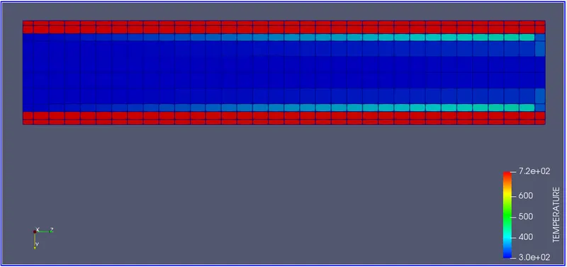
2.Temperature contour plot:
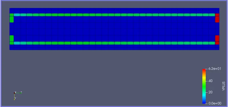
3.Y plus contour plot:
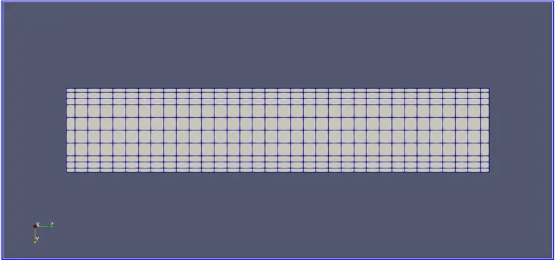
4.Mesh:
----------------------------------------------********************-----------------------------------------
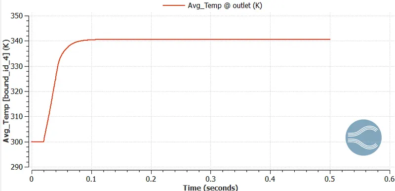
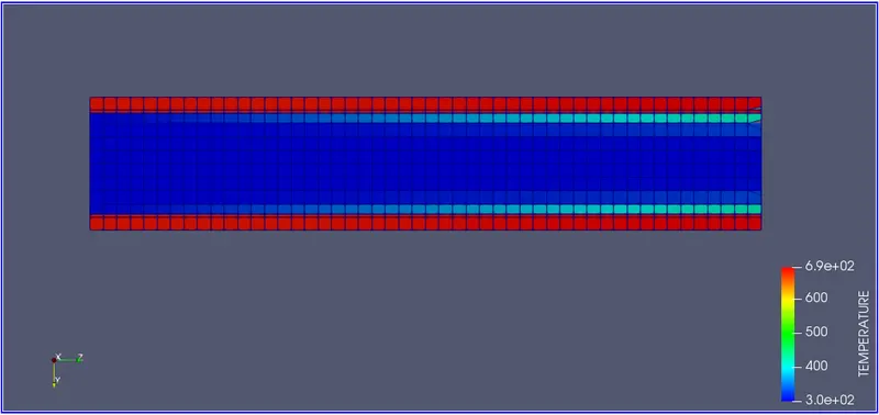
Case-4-->>Grid size-4 mm and Super cycling stage interval--0.01
1.Average Temperature @ Outlet line plot:
2.Temperature contour plot:
--------------------------------------------------*************----------------------------------------------
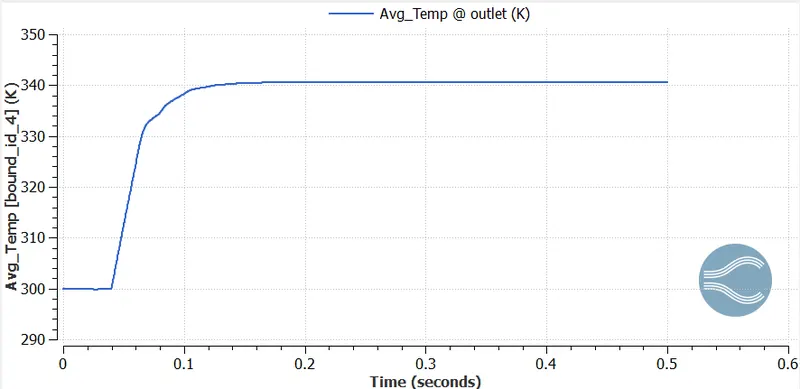
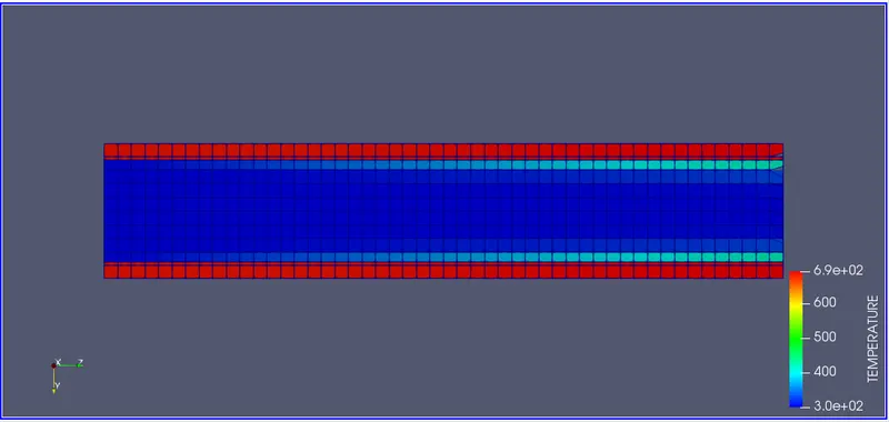
Case-5-->>Grid size-4 mm and Super cycling stage interval--0.02:
1.Average Temperature @ Outlet line plot:
2.Temperature contour plot:
----------------------------------------------****************----------------------------------------------
Case-6-->>Grid size-4 mm and Super cycling stage interval--0.03:
1.Average Temperature @ Outlet line plot:
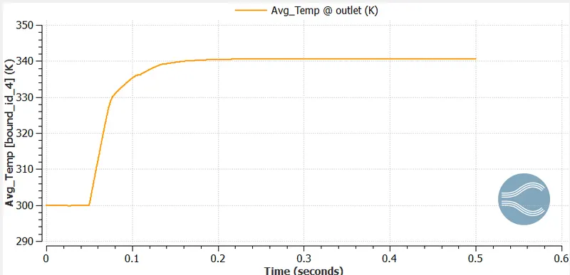
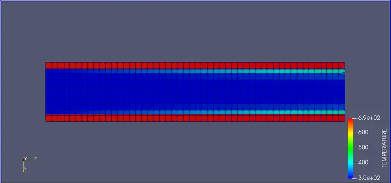
2.Temperature contour plot:
-------------------------------------------------*******************---------------------------------------
#Observations in Grid dependence test:
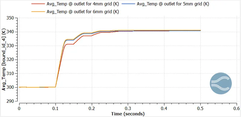
From the above plot we can observe that though grid size varied from 4 to 6 mm,but value for Temperature at the outlet obtained is almost close to each other.
Therefore it can be concluded that in this range of grid size,results are independent of grid.
---------------------------------------------------***********-----------------------------------------------
#Simulation time comparasion for different super cycling interval:
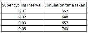
Super-cycling is a method used by CONVERGE Studio in the case of conjugate heat transfer problems with a solid and liquid regions.
Observation from the results were like,with the increase in super cycling interval simulation time also increases.
----------------------------------------------------*******************-----------------------------------
#Conclusion:
CHT analysis as we know is very important from maintaining particular temperature at outlets ,inlets of Heat exchangers,for analysis thermal stresses generating while heat transfer .
If thermal stresses developed on Heat exchanger body is more than the maximum limit of material (HE body) then that material at a point of time will fail due to stresses.
If designed Heat exchanger,is not able to maintain particular temperature for use in certain system in industries even after trying all possible ways of controlling flow through it,then there is no use of such Heat exchanger.
So before designing physical model of Heat exchanger points discussed above need to be keep in mind,which can be done by CHT analysis of a component.