Conjugate Heat Transfer Simulation
AIM
The aim of this simulation is to analyse the conjugate heat transfer through a cylinder
OBJECTIVES
- Flow simulation through pipe with conjugate heat transfer
- Turbulent flow with high Reynolds number
- Super cycle model needs to be implemented
CONJUGATE HEAT TRANSFER
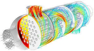
The term conjugate heat transfer (CHT) is used to describe processes which involve variations of temperature within solids and fluids, due to thermal interaction between the solids and fluids. The exchange of thermal energy between the two physical bodies is called study of Heat Transfer, the rate of transferred heat is directly proportional to the temperature difference between the bodies. A typical example is the heating or cooling of a solid object by the flow of air in which it is immersed and some other example includes conduction through solids, free and forced convection in the gases/fluids and thermal radiation.
Conjugate heat transfer corresponds with the combination of heat transfer in solids and heat transfer in fluids. In solids, conduction often dominates whereas in fluids, convection usually dominates. Efficiently combining heat transfer in fluids and solids is the key to designing effective coolers, heaters, or heat exchangers. Forced convection is the most common way to achieve high heat transfer rate. In some applications, the performances are further improved by combining convection with phase change (for example liquid water to vapor phase change).Heat transfer in solids and heat transfer in fluids are combined in the majority of applications. This is because fluids flow around solids or between solid walls, and because solids are usually immersed in a fluid.
Modes of heat transfer
- Conduction: diffusion of heat due to temperature gradients. A measure of the amount of conduction for a given gradient is the heat conductivity.
- Convection: when heat is carried away by moving fluid. The flow can either be caused by external influences, forced convection; or by buoyancy forces, natural convection. Convective heat transfer is tightly coupled to the fluid flow solution.
- Radiation: transfer of energy by electromagnetic waves between surfaces with different temperatures, separated by a medium that is at least partially transparent to the (infrared) radiation. Radiation is especially important at high temperatures, e.g. during combustion processes, but can also have a measurable effect at room temperatures.
An accurate description of heat transfer modes, material properties, flow regimes, and geometrical configurations enables the analysis of temperature fields and heat transfer.The fluid flow and heat transfer problems can be tightly coupled through the convection term in the energy equation and when physical properties are temperature dependent. While analytical solutions exist for some simple problems, we must rely on computational methods to solve most industrially relevant applications.CHT can be performed to improve cooling performance of the water jacket and increase engine life. Advancements in cooling for applications such as gas turbines components require improved understanding of the complex heat transfer mechanisms and the interactions between those mechanisms, which our engineers can perform without hassle. Critical cooling applications often rely on multiple thermal protection techniques, including internal cooling, external film cooling, etc. which are efficiently used by our analysis to cool components and limit the use of coolant. We do extensive support for Motor and Battery CHT Analysis to get optimized design for High voltage systems. Conjugate Heat Transfer analysis provides the temperature distribution in solid and coolant of the engine and clear insight on velocity distribution and mechanism of heat transfer of coolant. Results of CHT analysis become input to structural simulations as thermal loads.
CHT SIMULATION THROUGH PIPE
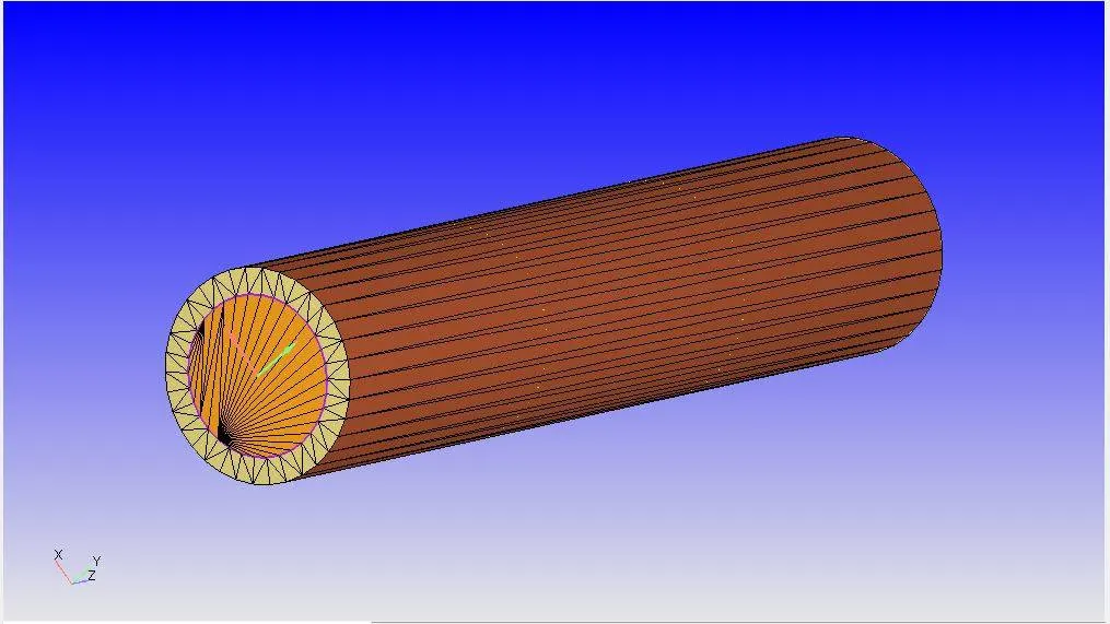
Geometry
Mesh
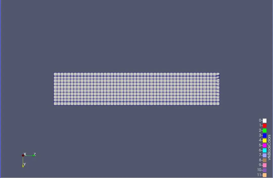
Computational mesh shows the base grid of 0.004m for the conjugate heat transfer simulation, the solid region and the fluid region can almost be visualised with the dark blue line. This lines helps in identification of both the regions
BOUNDARY CONDITIONS
Solid Outer Wall
- Temperature - flux type
- Heat Flux = -10000 `W/m^2`
- Velocity - No slip
Inlet
- INFLOW CONDITION
- Z-Velocity component (w) = 5.5 m/s
- Temperature = 300 K
- Mixture - Air
- Turbulence Model - K-epsilon
Outlet
- OUTFLOW CONDITION
- Pressure = 101325 `N/m^2`
- Temperature = 300 K
- Mixture - Air
Interface
- Forward Side - Fluid Region
- Reverse Side - Solid Region
Super Cycle Model
- Begin cycle = 0.01 s
- Solver - Steady state for Solid region
- Conduction CFL number = 100
- Resolution Factor = 1.4
Since we are modelling a turbulent flow problem, the Reynolds number is assumed to be 7000 in this case. The velocity which is supplied at the inlet is to be derived from the following formula
`Re=frac[vD][nu]`
`v=frac[nuxxRe][D}`
The following parameters are listed for air
- Kinematic viscosity @ 300 K = 15.69e-6 `m^2/s`
- Diameter of pipe = 0.02 m
- Reynolds Number = 7000
`v = frac[15.69e-6xx7000][0.02]`
`v = 5.5 m/s`
Results
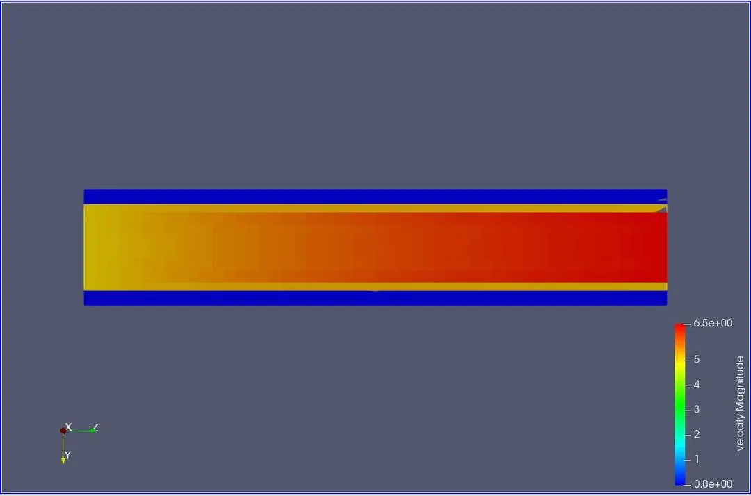
Velocity contour
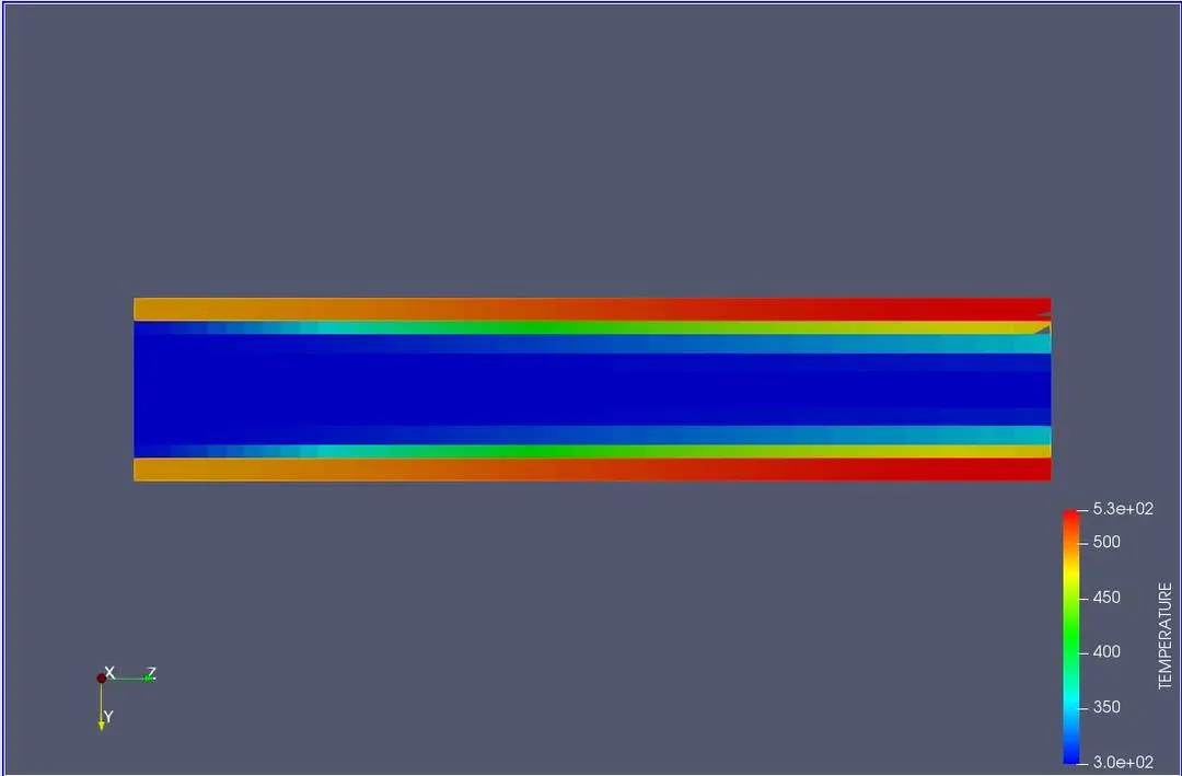
Temperature Contour
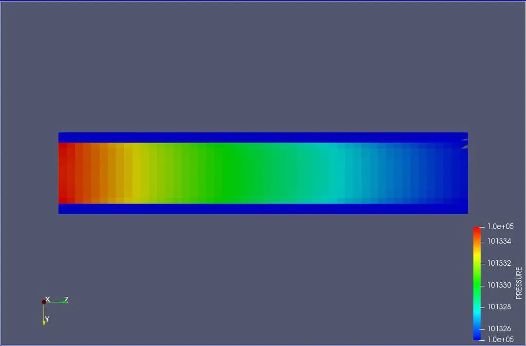
Pressure Contour
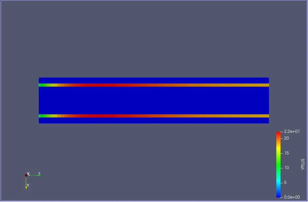
Y plus
Mass flow rate versus seconds
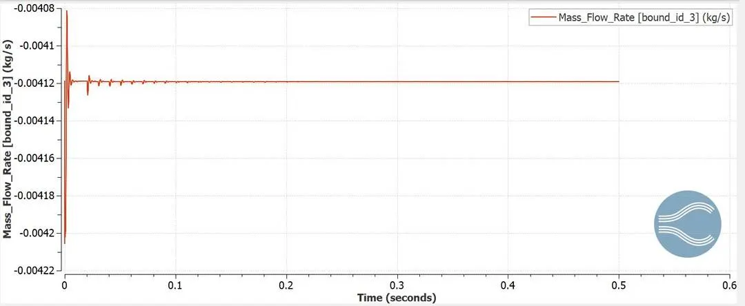
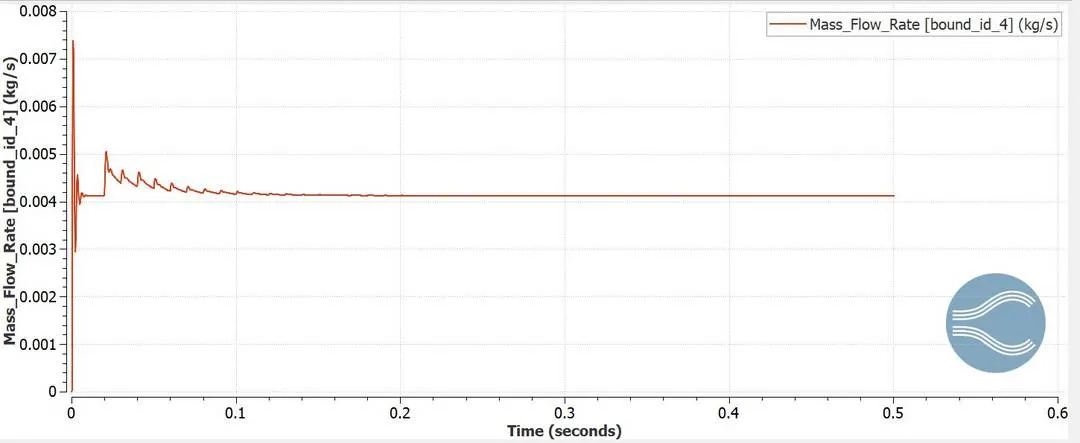
Since we can observe from both the above plots, there is mass flow rate of 0.00412 kg/s with both having opposite signs. This implies that the mass has been conserved.
Pressure versus seconds
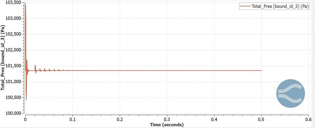
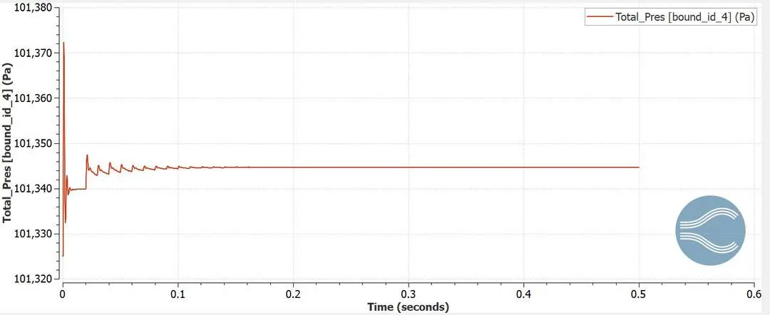
There is a small difference in the outlet and inlet pressure is 60 bar. Inlet pressure of 101,400 bar and the outlet pressure is somewhere around 101 344 bar. This is the driving agent for the flow to occur.
Temperature versus seconds
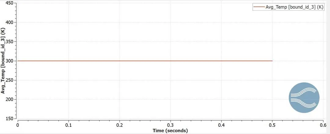
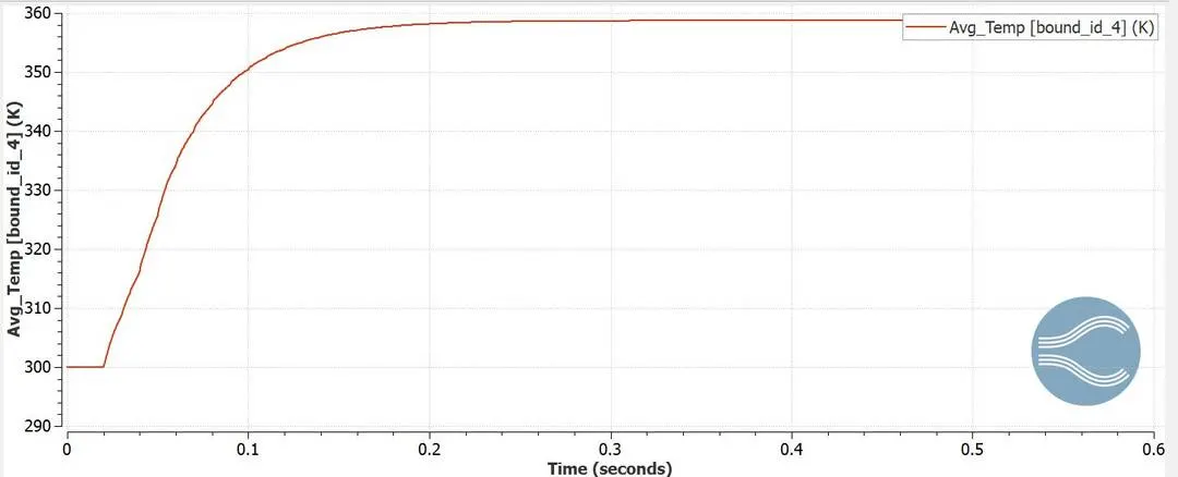
The inlet temperature is 300 K and outlet is 350 K. this rise in temperature is due to the heat flux which is provided in the boundary conditions.
Velocity versus seconds
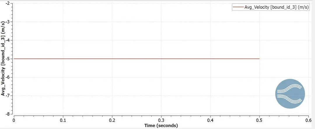
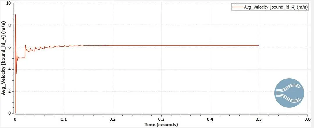
Finally the velocity reaches a steady state value of 6 m/s. At the inlet velocity is 5.5 m/s, but when the volume expand due to the heat supplied the velocity becomes 6 m/s
CHT SIMULATION THROUGH PIPE
Geometry
Mesh

Computational mesh shows the base grid of 0.003m for the conjugate heat transfer simulation, the solid region and the fluid region can almost be visualised with the dark blue line. This lines helps in identification of both the regions
BOUNDARY CONDITIONS
Solid Outer Wall
- Temperature - flux type
- Heat Flux = -10000 `W/m^2`
- Velocity - No slip
Inlet
- INFLOW CONDITION
- Z-Velocity component (w) = 5.5 m/s
- Temperature = 300 K
- Mixture - Air
- Turbulence Model - K-epsilon
Outlet
- OUTFLOW CONDITION
- Pressure = 101325 `N/m^2`
- Temperature = 300 K
- Mixture - Air
Interface
- Forward Side - Fluid Region
- Reverse Side - Solid Region
Super Cycle Model
- Begin cycle = 0.01 s
- Solver - Steady state for Solid region
- Conduction CFL number = 100
- Resolution Factor = 1.4
Since we are modelling a turbulent flow problem, the Reynolds number is assumed to be 7000 in this case. The velocity which is supplied at the inlet is to be derived from the following formula
`Re=frac[vD][nu]`
`v=frac[nuxxRe][D}`
The following parameters are listed for air
- Kinematic viscosity @ 300 K = 15.69e-6 `m^2/s`
- Diameter of pipe = 0.02 m
- Reynolds Number = 7000
`v = frac[15.69e-6xx7000][0.02]`
`v = 5.5 m/s`
Results
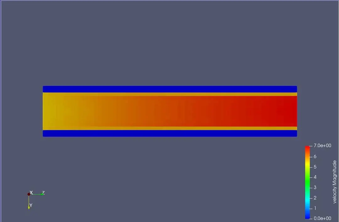
Velocity contour
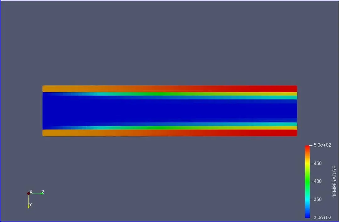
Temperature Contour
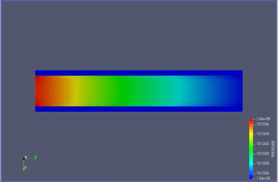
Pressure Contour
Y plus
Mass flow rate versus seconds
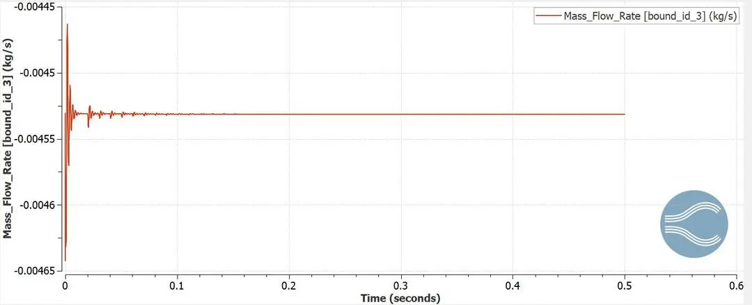
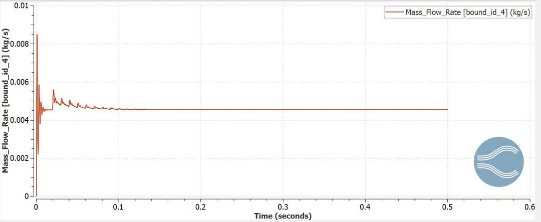
Since we can observe from both the above plots, there is mass flow rate of 0.004525 kg/s with both having opposite signs. This implies that the mass has been conserved.
Pressure versus seconds
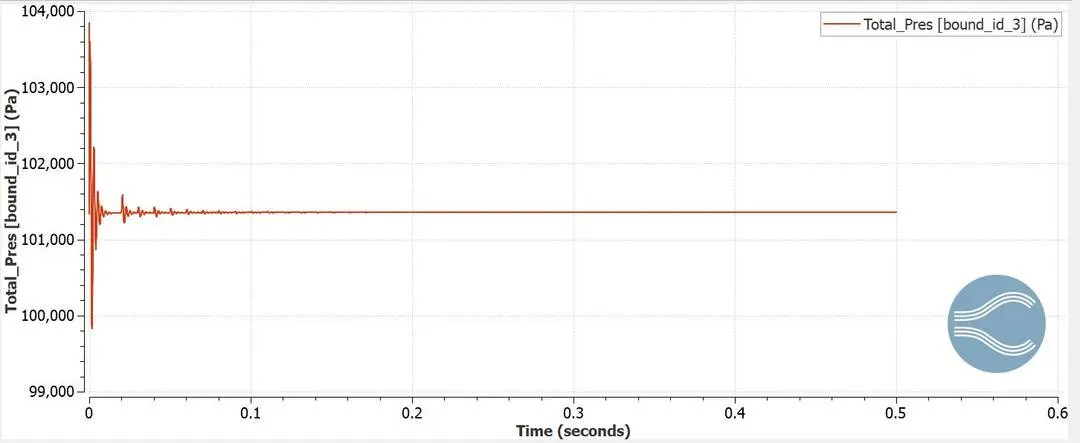
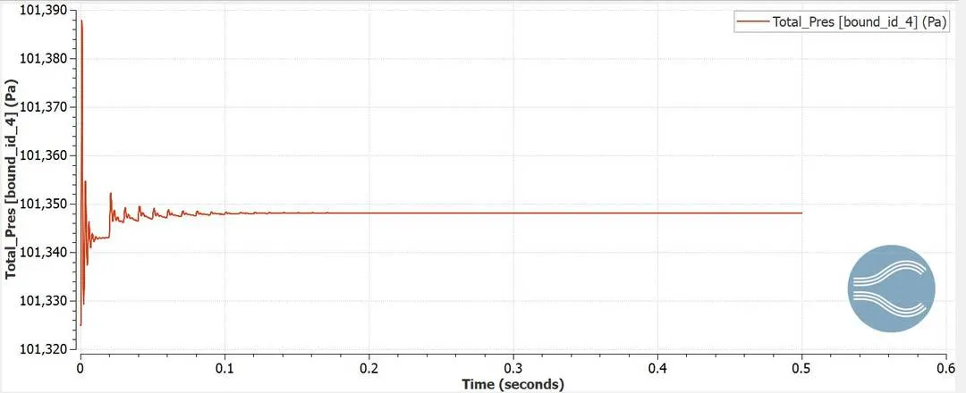
There is a small difference in the outlet and inlet pressure is 60 bar. Inlet pressure of 101,400 bar and the outlet pressure is somewhere around 101 348 bar. This is the driving agent for the flow to occur.
Temperature versus seconds
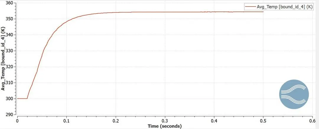
The inlet temperature is 300 K and outlet is 354 K. this rise in temperature is due to the heat flux which is provided in the boundary conditions.
Velocity versus seconds
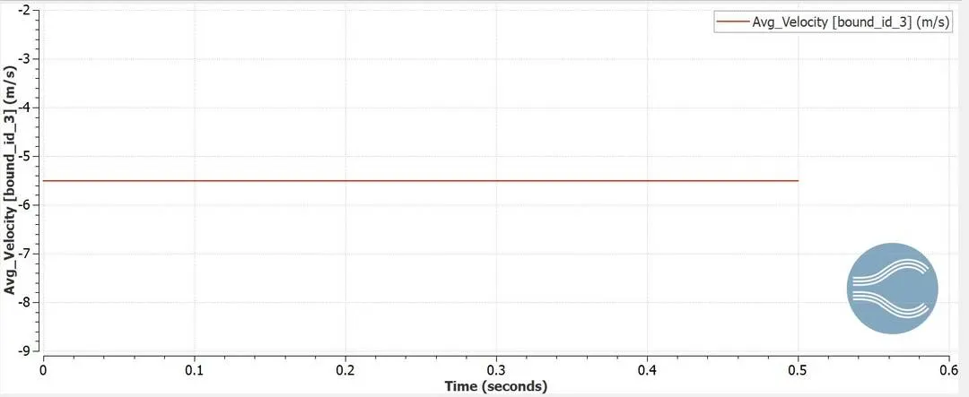
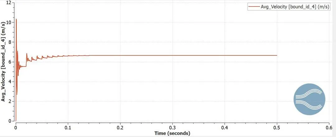
Finally the velocity reaches a steady state value of 6.5 m/s. At the inlet velocity is 5.5 m/s, but when the volume expand due to the heat supplied the velocity becomes 6.5 m/s
CHT SIMULATION THROUGH PIPE
Geometry
Mesh

Computational mesh shows the base grid of 0.002m for the conjugate heat transfer simulation, the solid region and the fluid region can almost be visualised with the dark blue line. This lines helps in identification of both the regions
BOUNDARY CONDITIONS
Solid Outer Wall
- Temperature - flux type
- Heat Flux = -10000 `W/m^2`
- Velocity - No slip
Inlet
- INFLOW CONDITION
- Z-Velocity component (w) = 5.5 m/s
- Temperature = 300 K
- Mixture - Air
- Turbulence Model - K-epsilon
Outlet
- OUTFLOW CONDITION
- Pressure = 101325 `N/m^2`
- Temperature = 300 K
- Mixture - Air
Interface
- Forward Side - Fluid Region
- Reverse Side - Solid Region
Super Cycle Model
- Begin cycle = 0.01 s
- Solver - Steady state for Solid region
- Conduction CFL number = 100
- Resolution Factor = 1.4
Since we are modelling a turbulent flow problem, the Reynolds number is assumed to be 7000 in this case. The velocity which is supplied at the inlet is to be derived from the following formula
`Re=frac[vD][nu]`
`v=frac[nuxxRe][D}`
The following parameters are listed for air
- Kinematic viscosity @ 300 K = 15.69e-6 `m^2/s`
- Diameter of pipe = 0.02 m
- Reynolds Number = 7000
`v = frac[15.69e-6xx7000][0.02]`
`v = 5.5 m/s`
Results
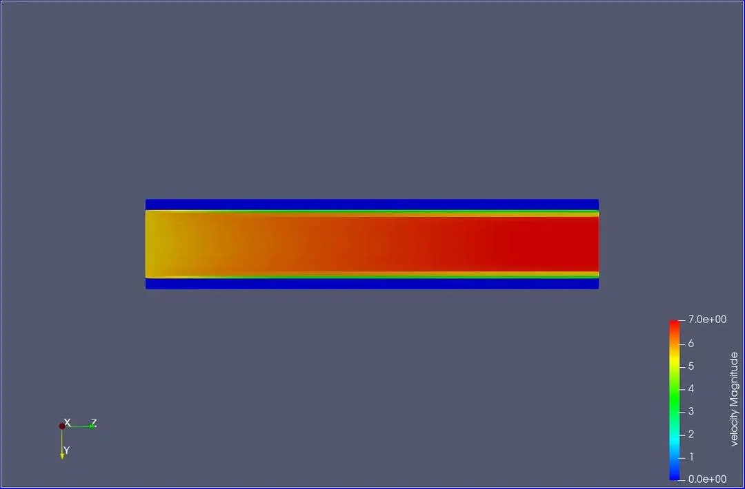
Velocity contour
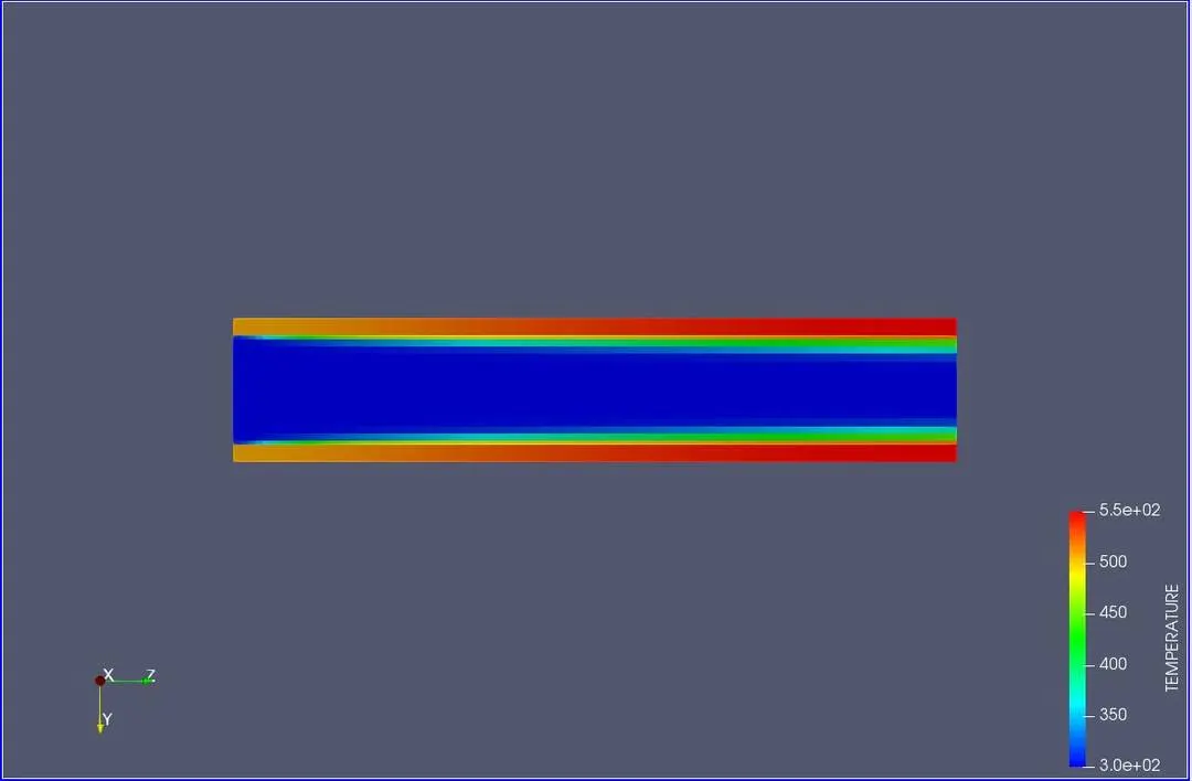
Temperature Contour
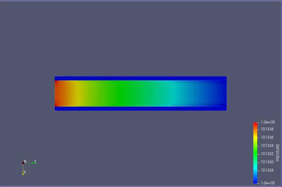
Pressure Contour
Y plus
Mass flow rate versus seconds
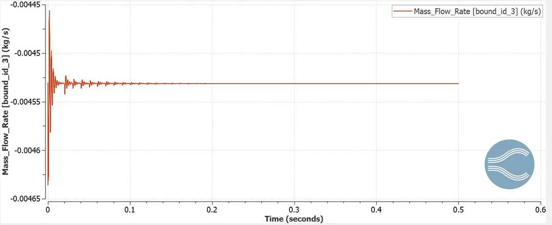
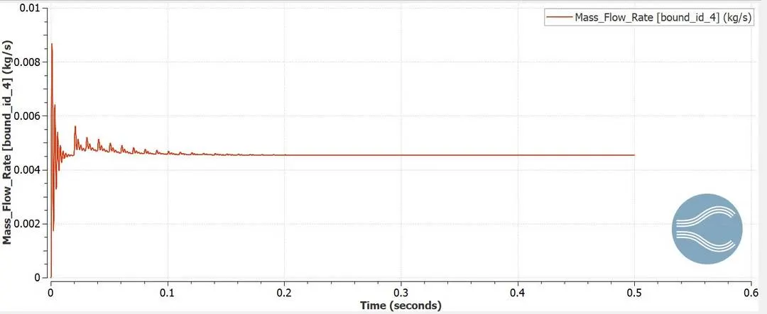
Since we can observe from both the above plots, there is mass flow rate of 0.004525 kg/s with both having opposite signs. This implies that the mass has been conserved.
Pressure versus seconds
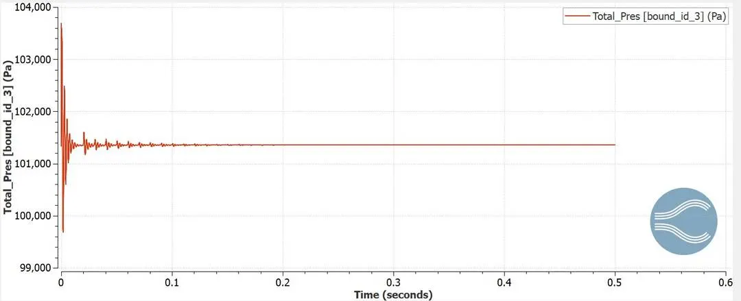
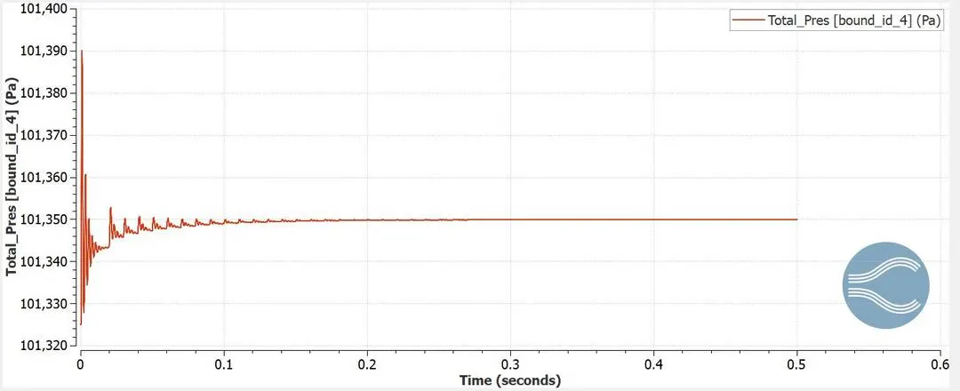
There is a small difference in the outlet and inlet pressure is 60 bar. Inlet pressure of 101,400 bar and the outlet pressure is somewhere around 101 344 bar. This is the driving agent for the flow to occur.
Temperature versus seconds
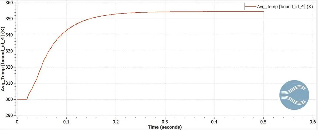
The inlet temperature is 300 K and outlet is 356 K. this rise in temperature is due to the heat flux which is provided in the boundary conditions.
Velocity versus seconds
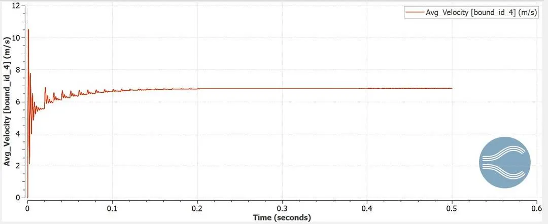
Finally the velocity reaches a steady state value of 7 m/s. At the inlet velocity is 5.5 m/s, but when the volume expand due to the heat supplied the velocity becomes 7 m/s
SUPER CYCLE MODEL
The internal combustion engine industry is moving toward simulating the entire system rather than independent components. Conjugate heat transfer (CHT)—the simultaneous prediction of heat transfer in both the fluid and solid portions of the domain—is of critical importance in a full-engine simulation. The accuracy of the predicted combustion in the cylinder is dependent on the temperature boundary conditions in the cylinder. By considering heat transfer in the metal components (e.g., the cylinder head, liner, piston, etc.) in the simulation, the cylinder wall no longer has a user-specified temperature, but instead has temperatures predicted as part of the system simulation. This makes the overall simulation results more predictive by reducing the dependence on boundary conditions.
There are several challenges when solving the fluid and solid domains together. The largest challenge to overcome is the difference in time-scales associated with the fluid and solid. In general, the heat transfer in the solid occurs more slowly than the convective and diffusive time-scales dictated by the fluid flow in the cylinder. For example, when you start a car in cold temperatures, combustion occurs almost instantly while the coolant takes minutes (thousands of cycles) to reach a steady-state temperature. This disparity in time-scales is problematic for CFD simulation because each cycle can be computationally expensive.
CONVERGE offers an alternative approach called super-cycling for overcoming the time-scale disparity. In super-cycling, the fluid solver is frozen periodically while the heat transfer in the solid is allowed to progress to steady-state. CONVERGE solves the fluid and solid phases in the same simulation without requiring you to stop and restart the simulation. Super-cycling significantly reduces the computational cost of the CHT simulation.
| Sl No | Super Cycle Interval(s) | Simulation Time(s) |
| 1 | 0.05 | 325 |
| 2 | 0.03 | 358 |
| 3 | 0.02 | 453 |
| 4 | 0.01 | 424 |
From the above table, it is clear that with increase in super cycle modelling interval, there is decrease in the simulation time.
GRID DEPENDENCY
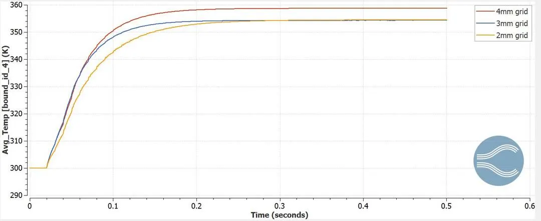
It is quite evident from the plot that the temperature has converged to a steady state value despite having different grid sizes or mesh size. This implies that the solution is Grid Independent.
TEMPERATURE ANIMATION
CONCLUSION
- Turbulent Flow across a pipe was simulated with conjugate heat transfer
- Grid dependency test shows the solution is not grid dependent
- Super cycle model is used for CHT