Conjugate Heat Transfer Simulation
Aim: To setup the case and perform conjugate heat transfer simulation for flow through the pipe with the help Converge CFD software.
Objective: 1. To setup case for flow through the pipe whose inlet reynolds number is equal to 7000
2. To perform a grid dependance test for three different grid size.
3. To study the effects of super cycle stage interval in CHT simulations.
4. To observe the changes of y-plus parameter for different grid size.
Introduction:
When heat transfer takes place simultaniously within and between the fluid and solid regions, the phenomenon is called as conjugate heat transfer. The main mode of heat transfer in fluids is convection while the main mode of heat transfer in solid is conduction. Typical applications where CHT analysis is performed are simulation of heat exchangers, cooling of electronic equipments and general purpose cooling and heating.
In this project, the CHT analysis for flow through a pipe with outer diameter 0.02 m and inner diameter 0.015 and with reynolds number equal to 7000 is performed. The part 1 of the simulation deals with the grid dependency test, where the grid size is varied until the convergence of desired output parameter is independent of the grid size. The part 2 of simulation deals with the effect of super cycle stage interval on the CHT analysis. And in both parts of the simulation, the effect of grid size on the y-plus parameter is studied.
What is super cycle modeling ?
The time scale for the solid phase heat transfer is larger than the time scale for the fluid phase heat transfer. Hence, it is not practical to perform CHT simulation simulataniously. The converge CFD software offers super cycle modeling where the solver calculates heat transfer at solid region and fluid region periodically. The converge solves both the equations of fluid and solid regions together initially using transient solver. At time equal to super cycle start time+super cycle stage interval time, the converge freezes fluid solver and solid heat transfer calculation is done. Once the solid heat transfer calculation is sompleted and the time is greater than super cycle stage interval, the fluid solver is resumed and this cycle is repeated until the end time of the simulation.
What is Y plus ?
The y-plus is a dimensionless parameter which helps in determining the first cell height from the wall. The behaviour of flow near the wall is a complex phenomenon and y-plus helps to distinguish the different regions near the wall.
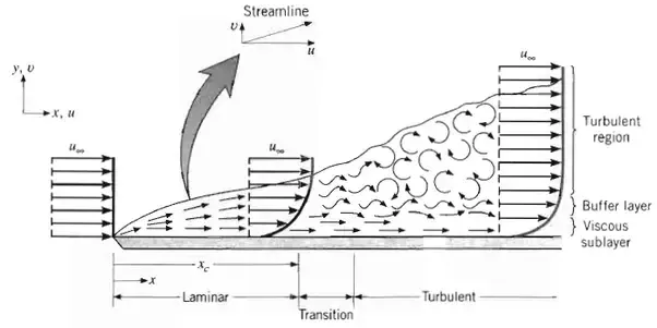
From the above figure, it can be seen that flow is laminar at the start and then transition at a certain distance and finaly the flow becomes turbulent. The y-plus parameter helps in determining the cell location in these regions.
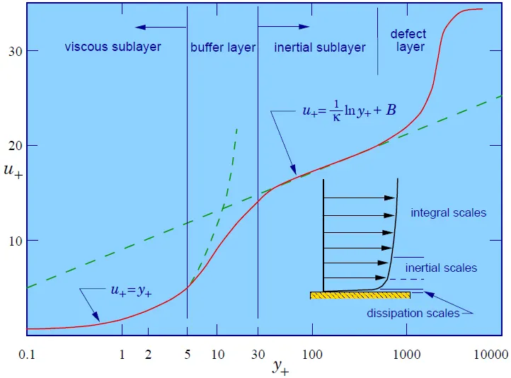
The above graph shows the various values of y-plus for different regions in the boundary layer. For simulation with heat transfer calculation it is desirable to have y-plus value < 30 (in buffer layer or viscous sublayer). The near wall modeling impacts the solution accuracy, as the walls are the main source for vorticity and turbulence. In the near wall region the solution variables has large gradients. Therefore, accurate representation of flows near the wall gives accurate solution.
Case setup of CHT simulation for flow through pipe
Geometry of the pipe:
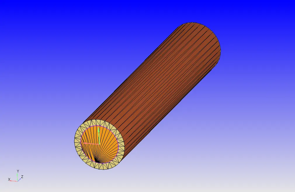
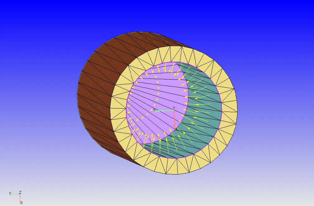
Normals direction pointing towards fluid domain
Boundary conditions:
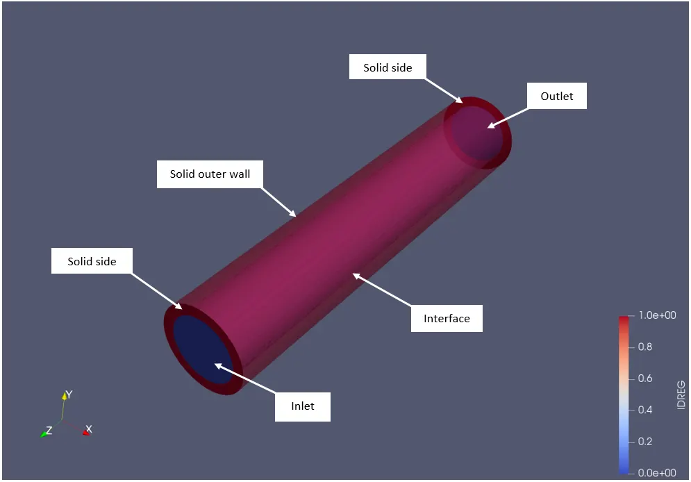
Inlet
Boundary type = inflow
Pressure = zero gradient (Neumann boundary condition)
Temperature = 300 K
Calculating velocity at inlet whose reynolds number is 7000
Re = (rho*V*d)/(Dynamic viscosity)
where,
rho-density of fluid (air)
V-velocity of fluid (air)
d-characteristic length (inner diameter of pipe)
V = (7000*1.849e-5)/(1.184*0.015) = 7.2877 m/s
Velocity = 7.2877 m/s (Dirichlet boundary condition)
Species = air
Outlet
Boundary type = outflow
Pressure = 101325 Pa
Temperature = 300 K
Species = air
Solid outer wall
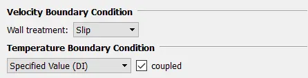
Boundary type = wall with slip condition
Wall motion type = stationary
Temperature = -10000 w/m2 (Heat flux)
Solid side
Boundary type = wall with slip condition
Wall motion type = stationary
Temperature = zero gradient (Neumann boundary condition)
Interface
Boundary type = interface
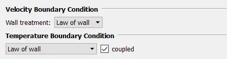
Forward side
Reverse side
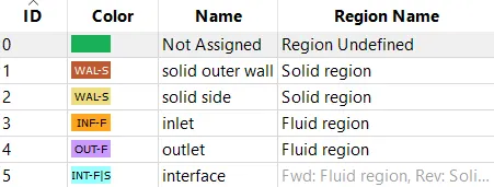
Assigning volumetric regions to boundaries
region 1 = Fluid region
Stream ID = 0
Temperature = 300 K
Pressure = 101325 Pa
Species = air
region 2 = Solid region
Stream ID = 1
Temperature = 300 K
Solid option - enabled
Species = Aluminium (mass fraction 1)
Simulation parameters
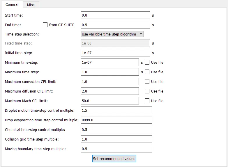
Solver type = transient state pressure based solver
Solver scheme = PISO
Turbulence model = K-epsilon
Super cycle model
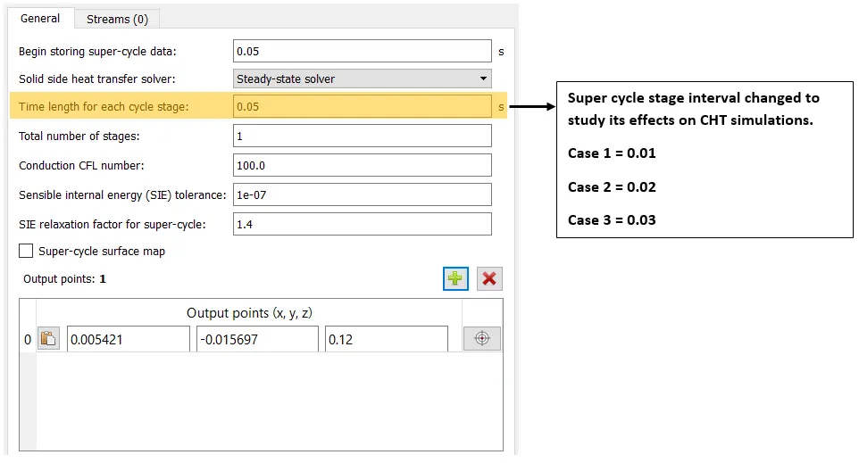
The geometry and case setup remains same for both parts of the simulation. Two regions are created as the simulation involves heat transfer calculation between two phases (fluid and solid). The air is added as the species for gas simulation and aluminium is added as species for solid simulation. The fluid and solid region is flagged to the respective boundaries. The fluid velocity at inlet is 7.2877 m/s which is calculated from the given reynolds number (7000). The slip boundary condition is used for walls in solid region where the stress tensor is set to zero. The law of wall boundary condition is used for walls in fluid region where the viscous sublayer needs to be resolved. The heat flux of -10000 w/m2 is added to the solid outer wall, where the heat transfer takes place across the entire surface of the solid outer wall boundary and the negative flux indicates that the heat flows into the domain. The interface boundary is used which allows to set up wall boundary that will separate regions and allows for interaction between two phase. The fluid region is used as forward side and solid side is used as reverse side. The regions in forward and reverse side is determined based on the normal vector direction. In this case, as the normals are pointing towards the fluid region it is used as forward side and as the normals are pointing away from the solid side it is used as the reverse side. The k-epsilon model is used for turbulence modeling ans super cycle model is used which helps in calculating the solid heat transfer by using steady state solver and transient solver seperately for fluid region. This way faster solution convergence is achived. The mesh generated and resuts obtained are discussed below.
Part 1 of simulation
Grid dependance test :
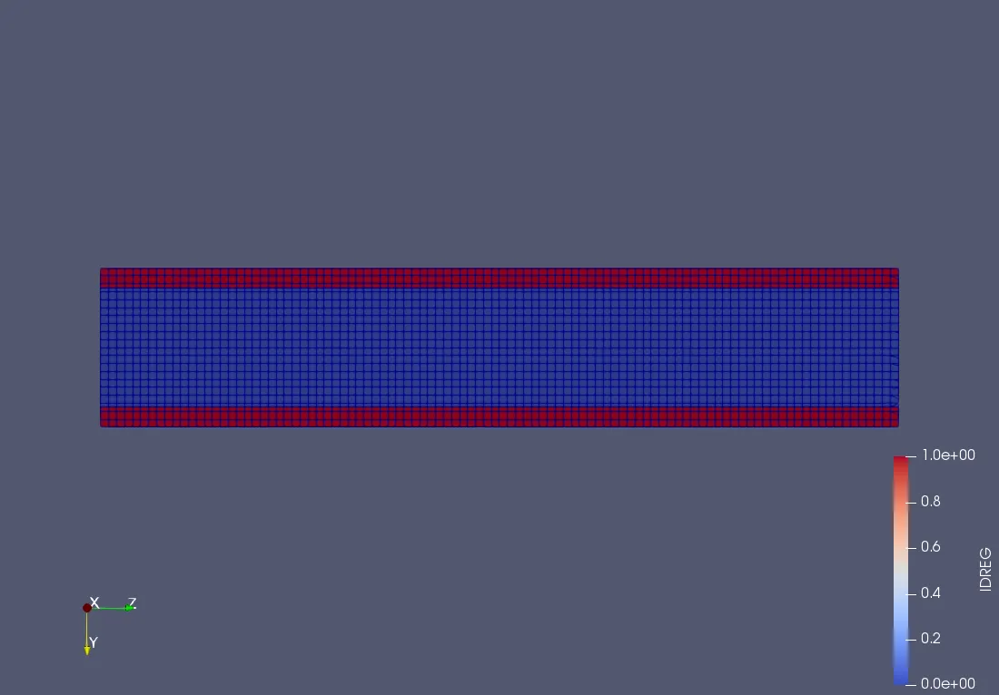
Comparing the mesh generated for different base grid size
Base grid size = 2.5 mm
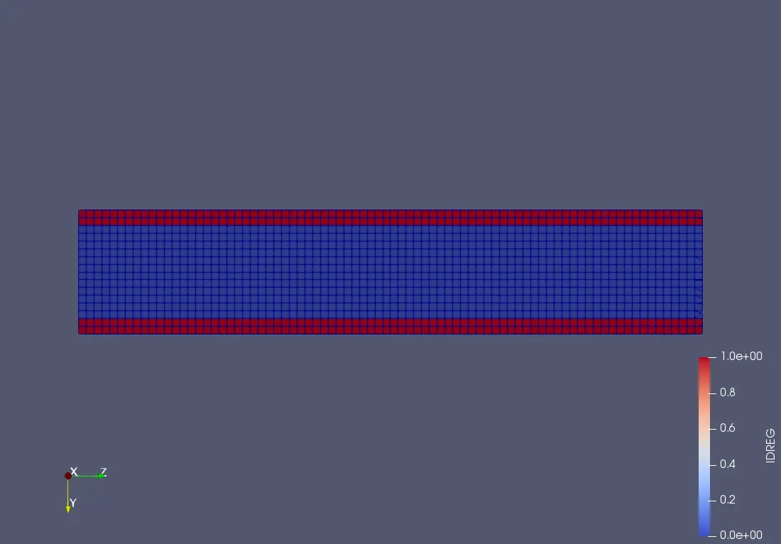
Base grid size = 2 mm
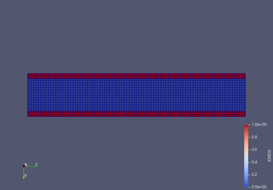
Base grid size = 1.5 mm
Results for grid size = 2.5 mm
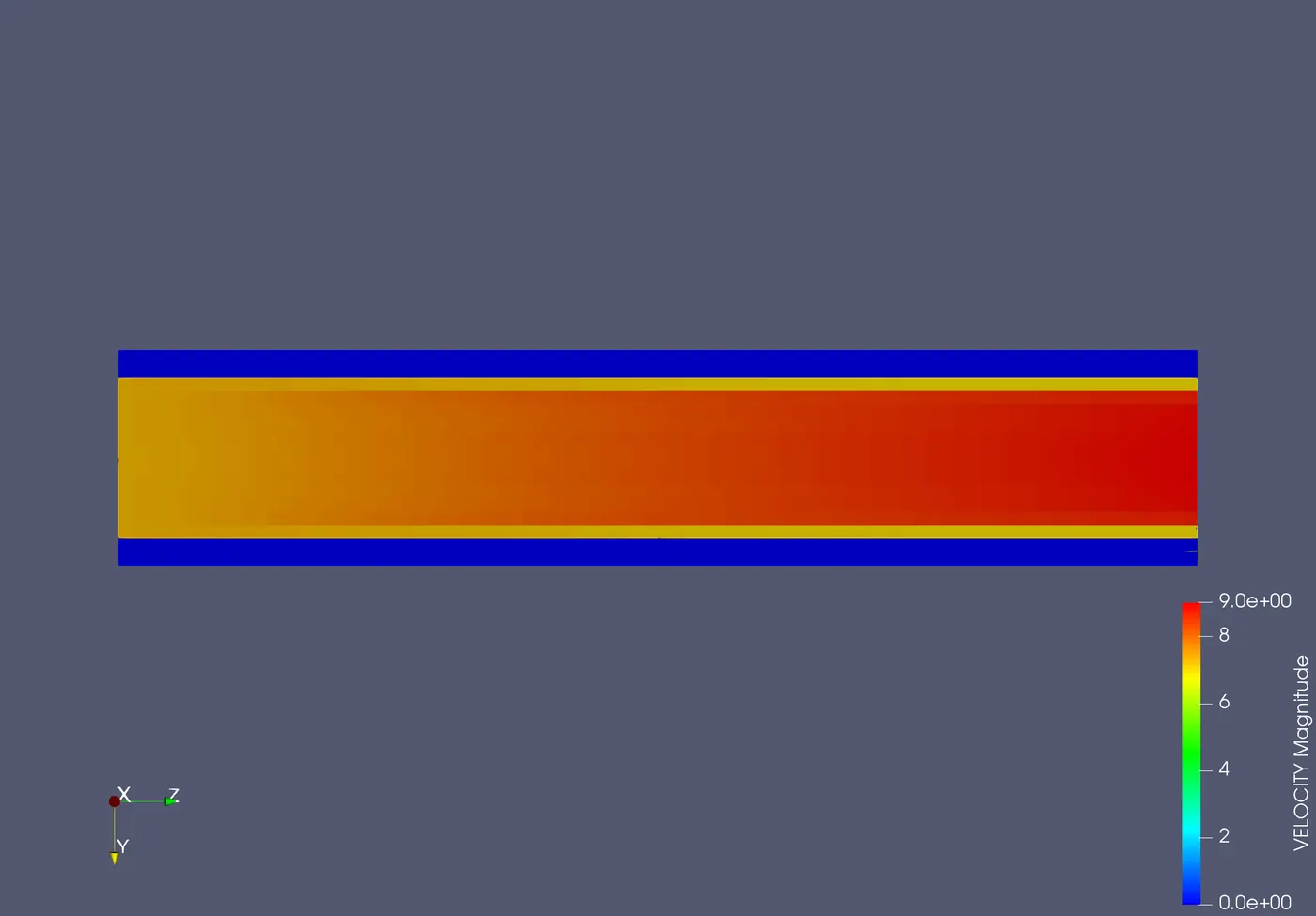
Velocity contour
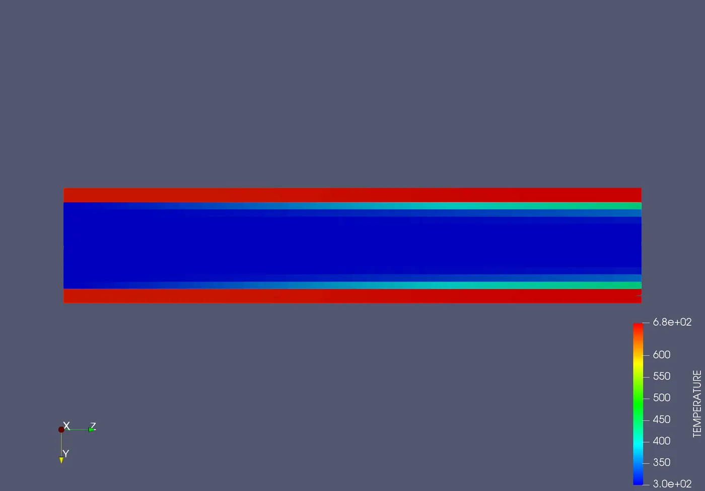
Temperature contour
Temperature animation
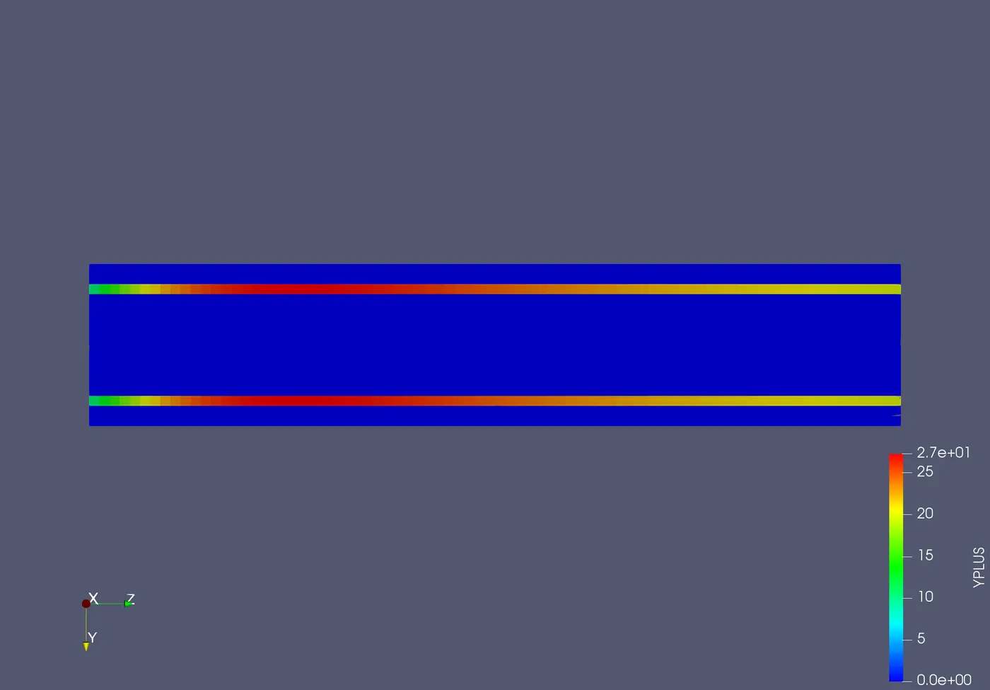
Y plus
Results for grid size = 2 mm
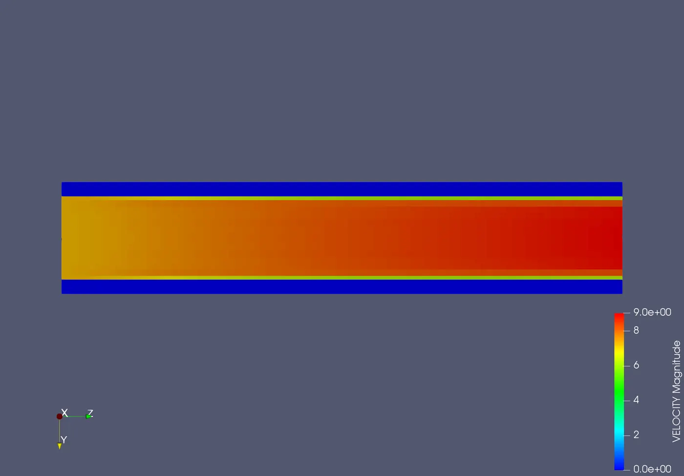
Velocity contour
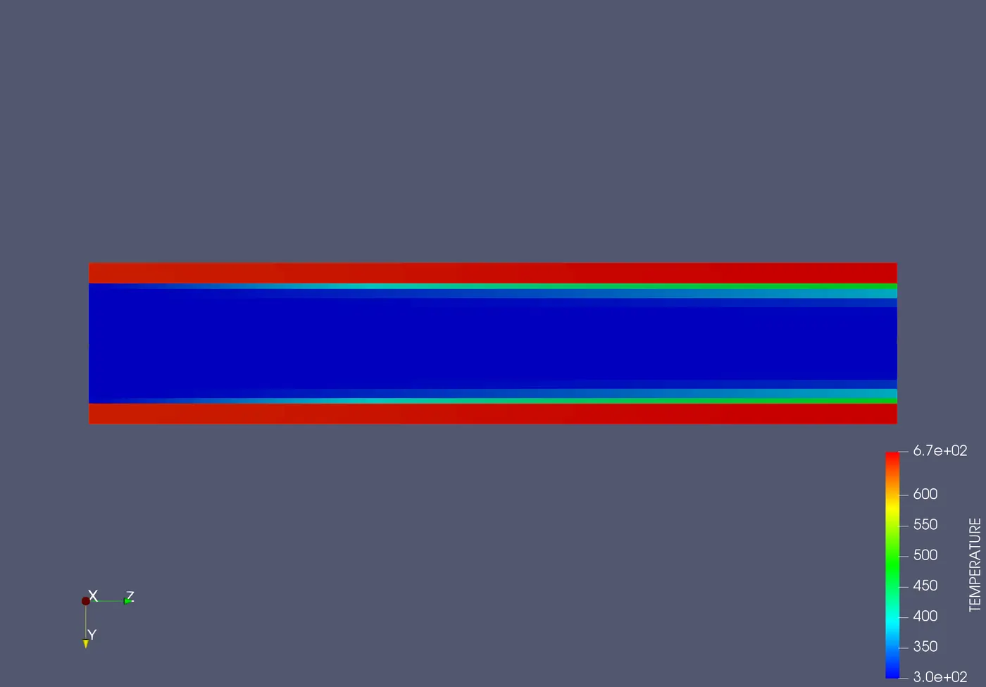
Temperature contour
Temperature animation
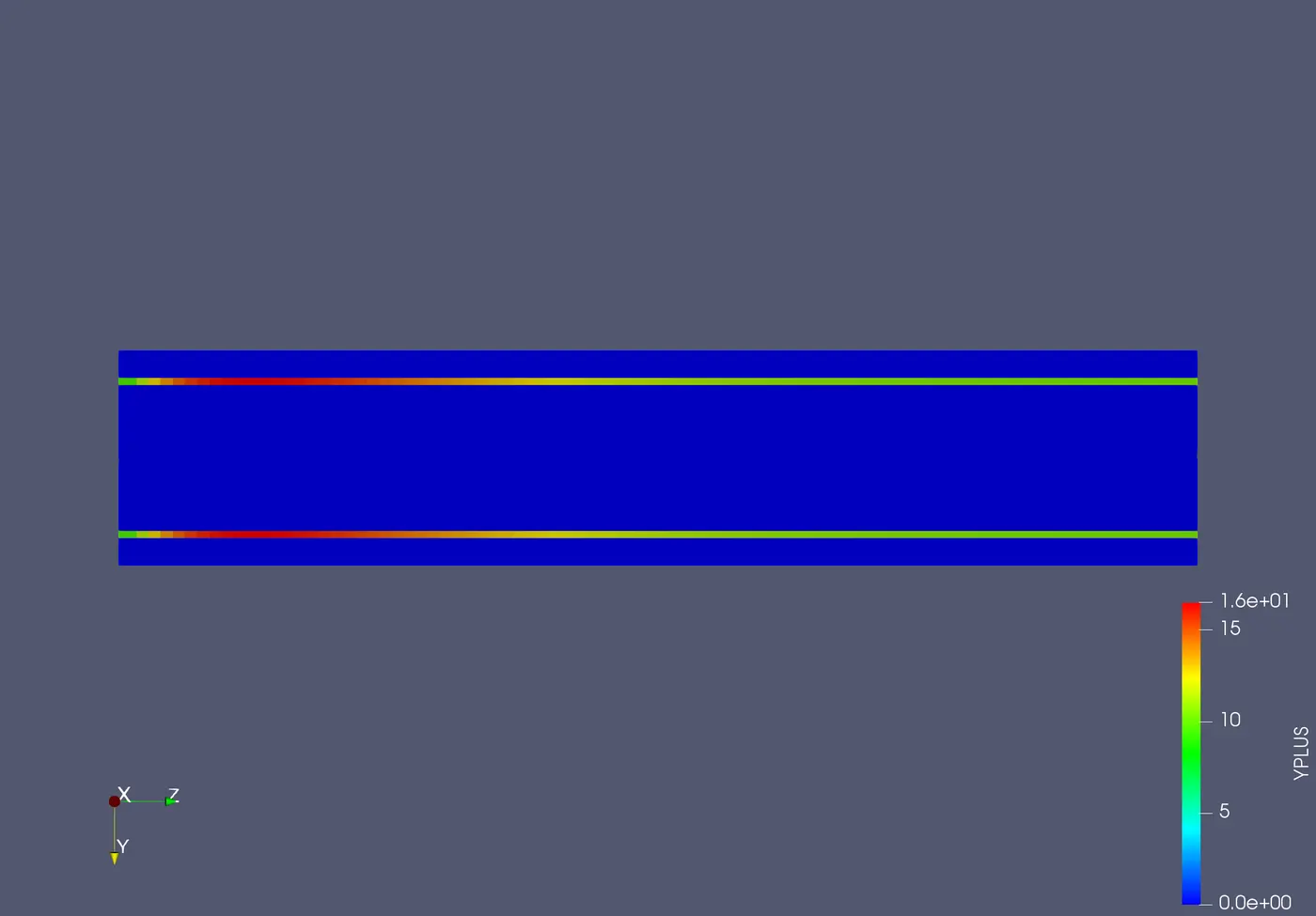
Y plus
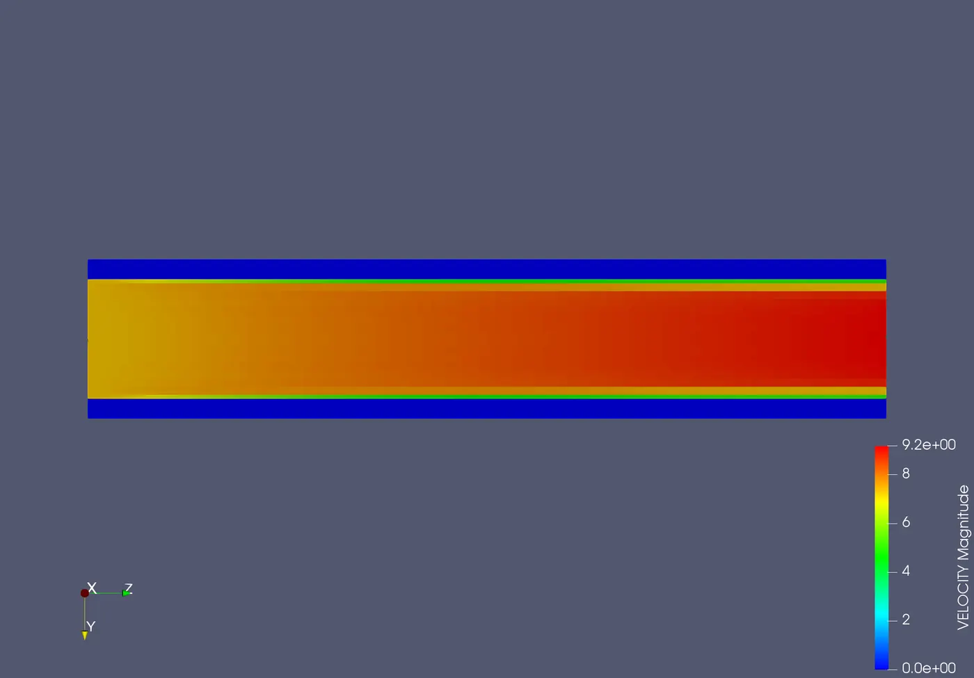
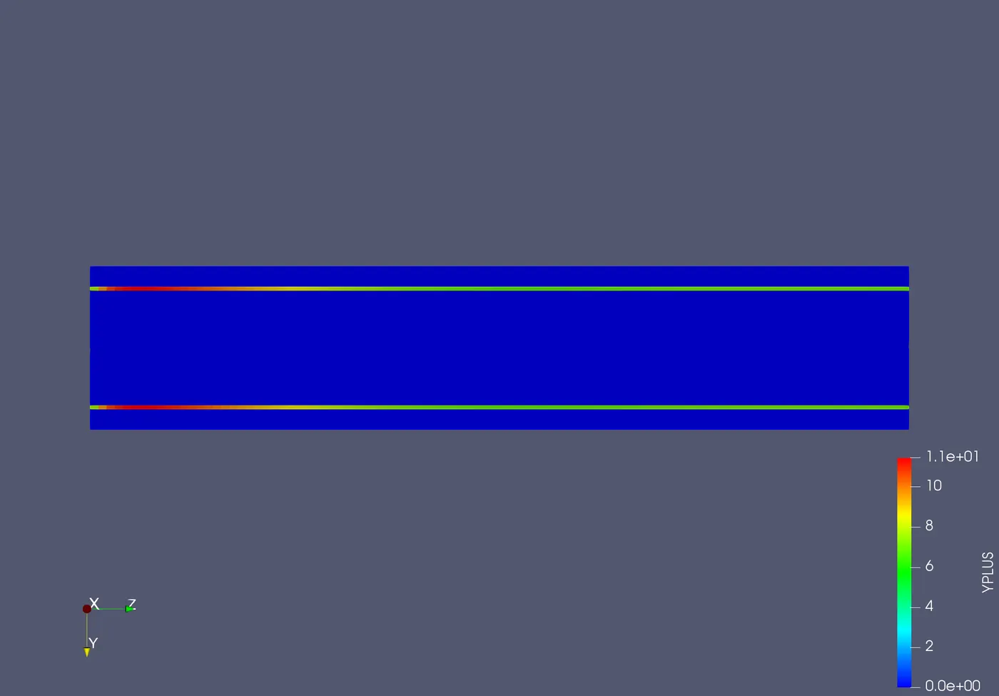
Result for grid size = 1.5 mm
Veocity contour
Temperature contour
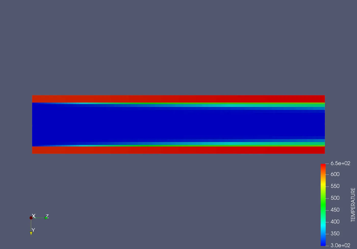
Temperature animation
Y plus
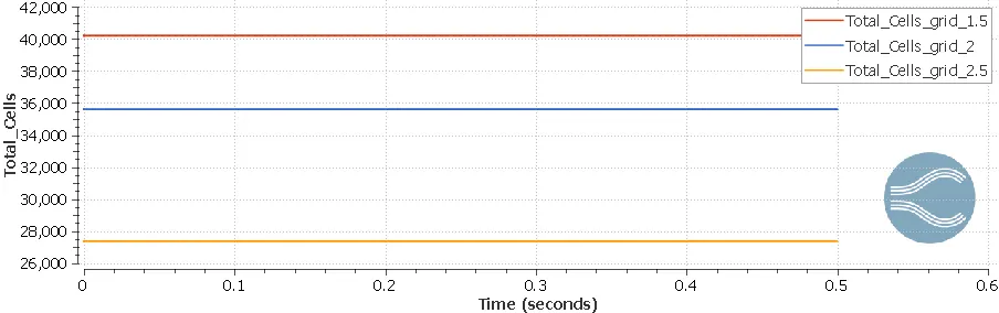
Cell count for different grid size
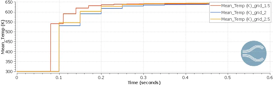
Comparing the mean temperature of solid region of different grid size
Comparing the mean temperature of fluid region of different grid size
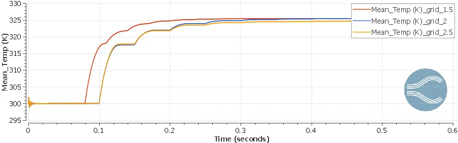
Obsvation from the part 1 of simulation
1. More cells are generated as the grid size is decreased hence, clear contours are obtained for lower grid size.
2. The mean temperature of solid region for grid size = 1.5 mm is 639.96 K, for grid size = 2 mm is 637.96 K and for grid size = 2.5 mm is 644.01. Thus less variation of temperature values is observed as grid size is changed.
3. The mean temperature of fluid region for grid size = 1.5 mm is 325.39 K, for grid size = 2 mm is 325.4 K and for grid size = 2.5 mm is 324.59 K.
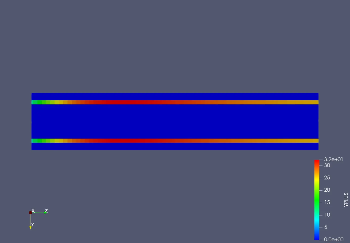
4. The y-plus values decreases as the grid size is decreased. The y-plus for grid size = 2.5 mm is 27, for grid size = 2 mm is 16 and for grid size = 1.5 mm is 11.
Part 2 of simulation
Effects of super cycle stage interval (SSI) on CHT simulation
Case 1 (SSI = 0.01)
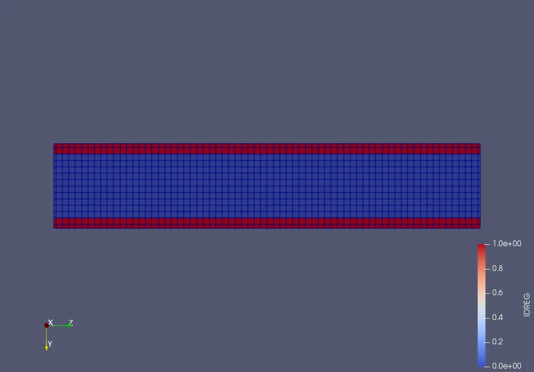
Mesh generated for grid size = 3 mm
Time taken by the solver in cygwin

Result for case 1
Velocity contour
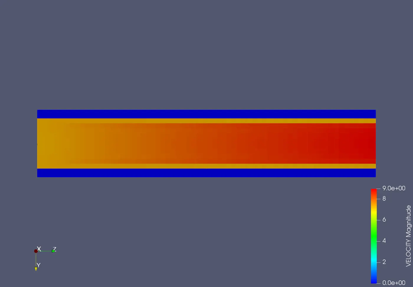
Temperature contour
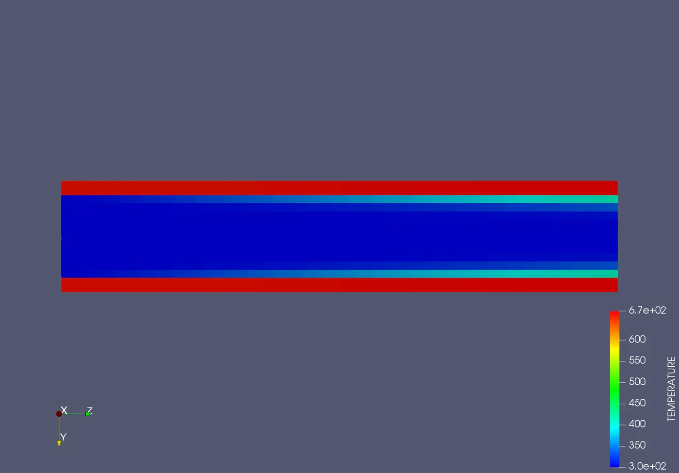
Y plus
Case 2 (SSI = 0.02)
Mesh generated for grid size = 3 mm
Time taken by solver in cygwin

Result for case 2
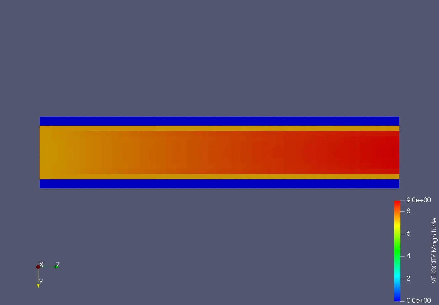
Velocity contour
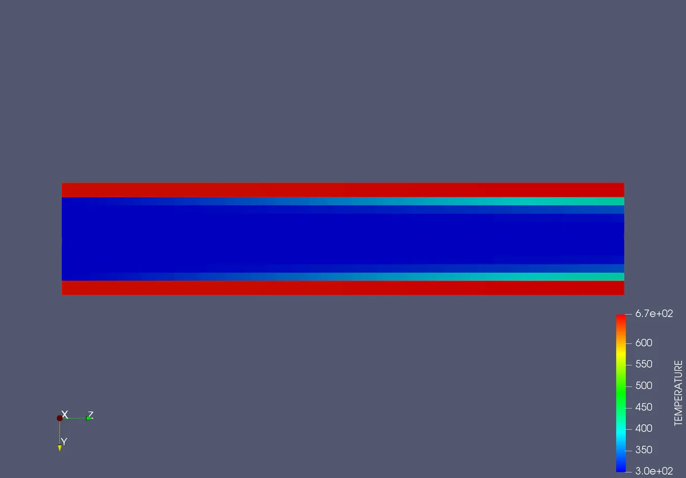
Temperature contour
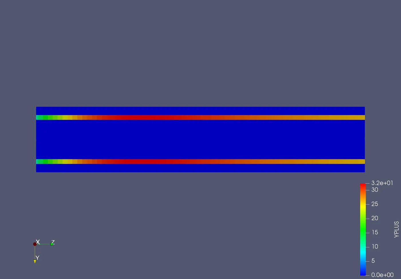
Y plus
Case 3 (SSI = 0.03)
Mesh generated for grid size = 3 mm
Time taken by solver in cygwin

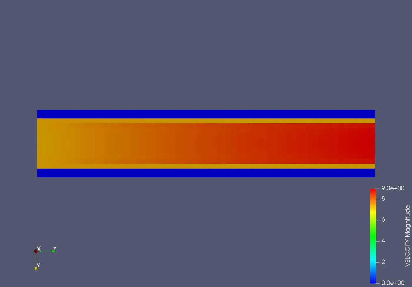
Velocity contour
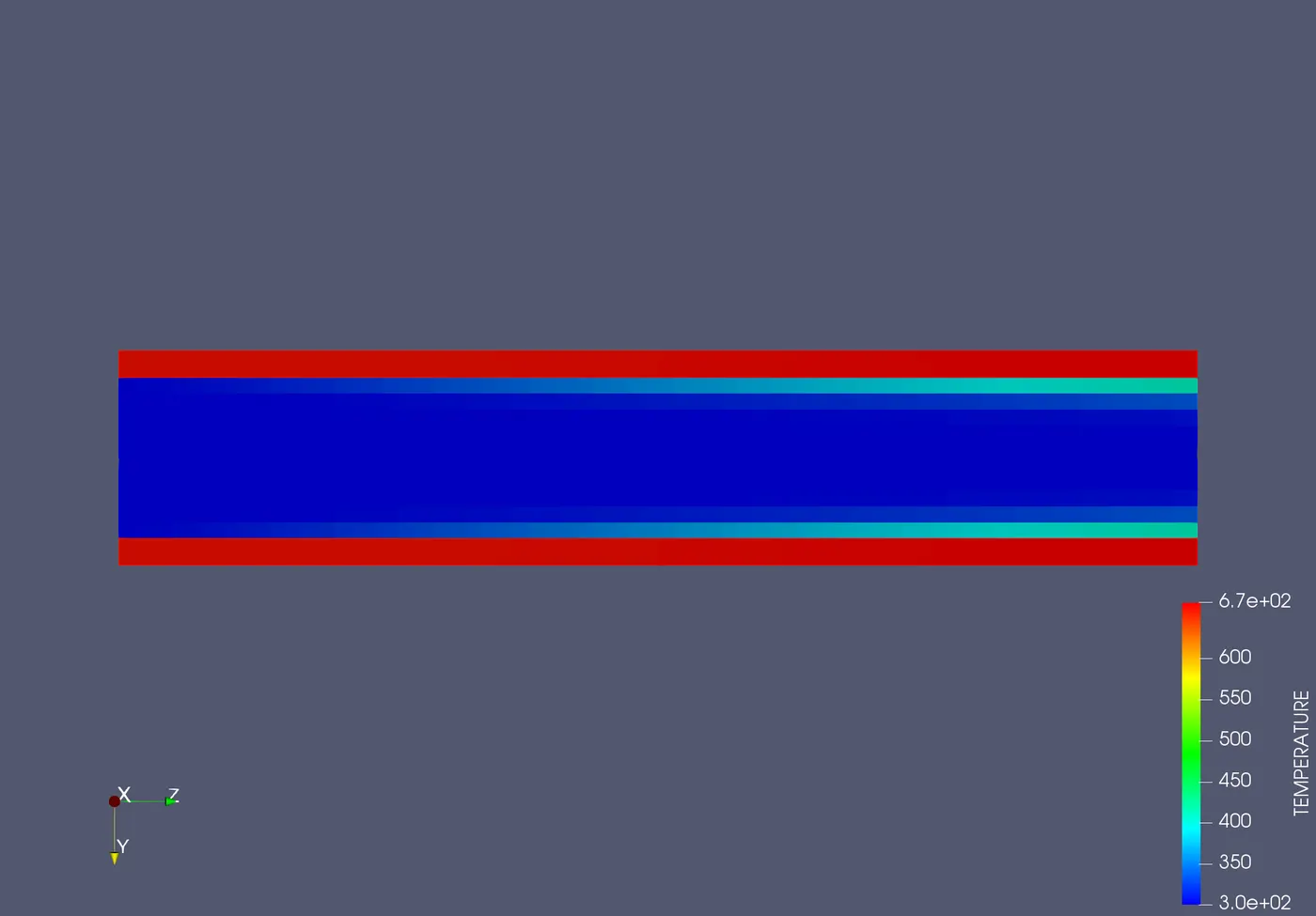
Temperature contour
Y plus
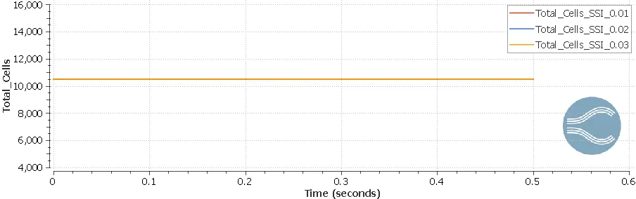
Cell count from all three cases
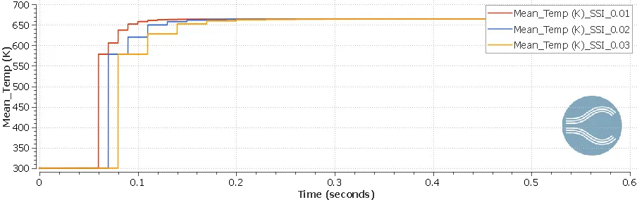
Comparing the mean temperature of solid region from all three cases
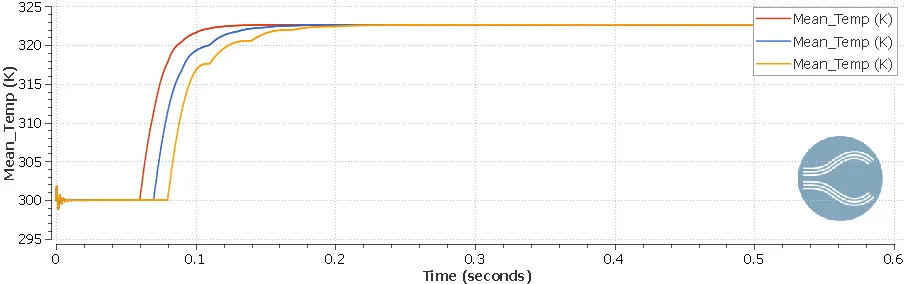
Comparing the mean temperature of fluid region from all three cases
Observation from part 2 of simulation:
1. The mean temperature of solid region converges to 664.024 K for the grid size 3 mm.
2. The mean temperature of fluid region converges to 322.631 K for the grid size 3mm.
3. The case 1 with super cycle stage interval 0.01 s reaches steady state early compared to other cases.
Conclusion:
The part 1 of simulation shows that further mesh refinement has to be done to get grid independant temperature values as slight variation is observed in the mean temperature values of solid region and fluid region for different grid size. The y-plus value decreases as the cell size near the wall is decreased. The part 2 of simulation shows that lower super cycle stage interval achives steady state faster. Therefore, lower super cycle stage interval reaches steady state faster.