Week 6: Conjugate Heat Transfer Simulation
AIM:
To Setup a flow simulation through a pipe Using Conjugate Heat Transfer simulation.
Given:
- Inlet Reynolds number should be 7,000
HINT : Use the below formula to calculate velocity for corresponding value of REYNOLD NUMBER and give DIRICHLET BC for velocity at inlet and specify the value for velocity calculated at INLET BC using below formula ,
Re = (rho*V*D)/(Dynamic viscosity)
- Turbulence modelling - K-Epsilon
- Supercycling parameters - same as in the video
- Set supercyle stage interval to 0.01,0.02 and 0.03
Objective:
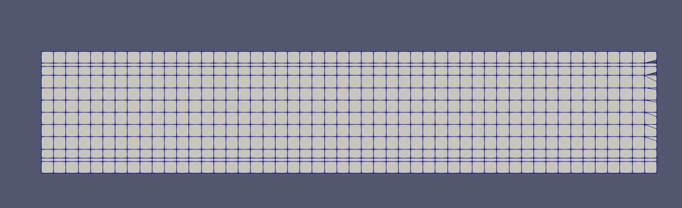
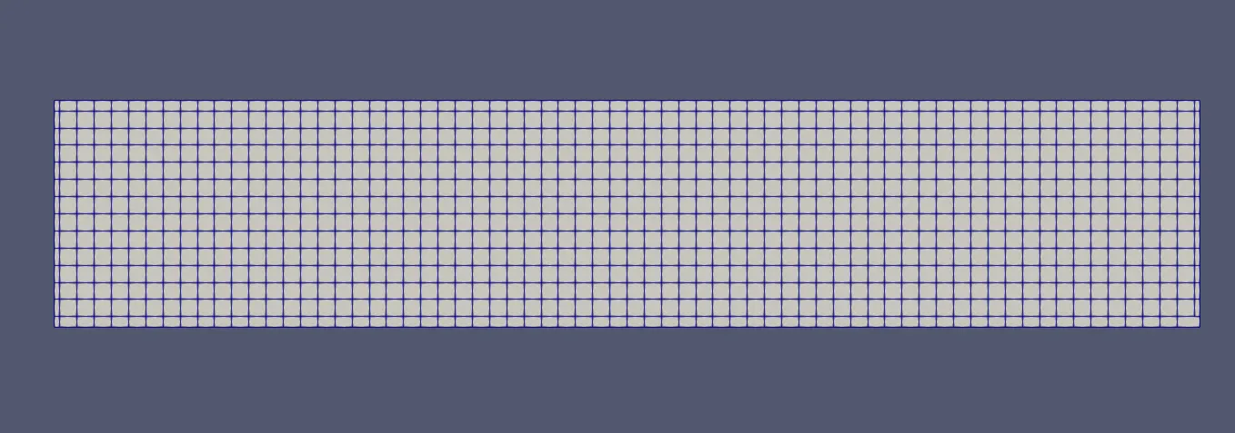
1. To Show the mesh for all the 3 base mesh sizes
2. Run grid dependence test on 3 grids and show that the outlet temperature converges to a particular value
3. Effect of supercycle stage interval
Procedure:
Step:1
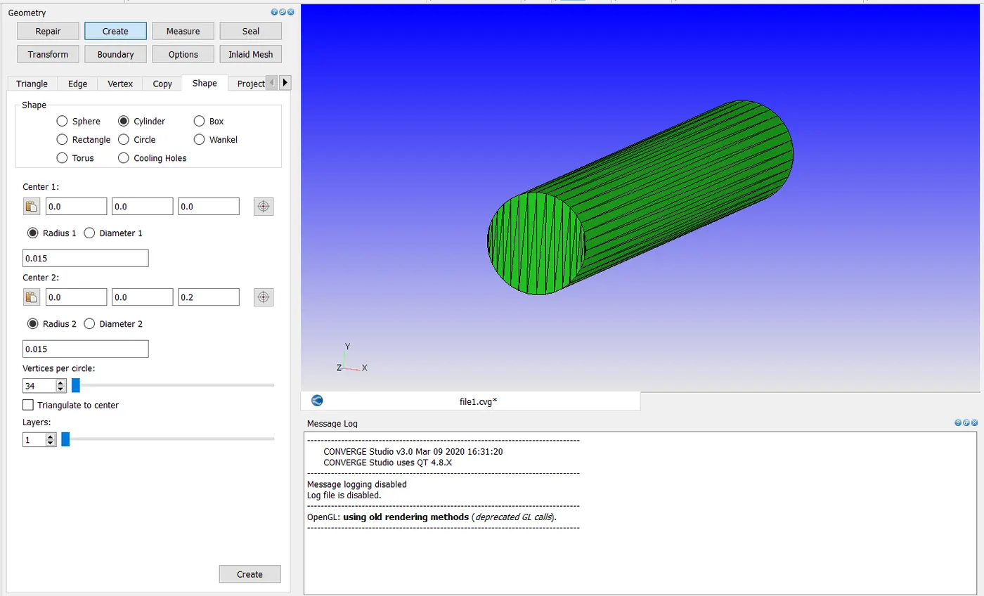
Create geomentry by shape option click cylinder and give the radius as shown in fig.
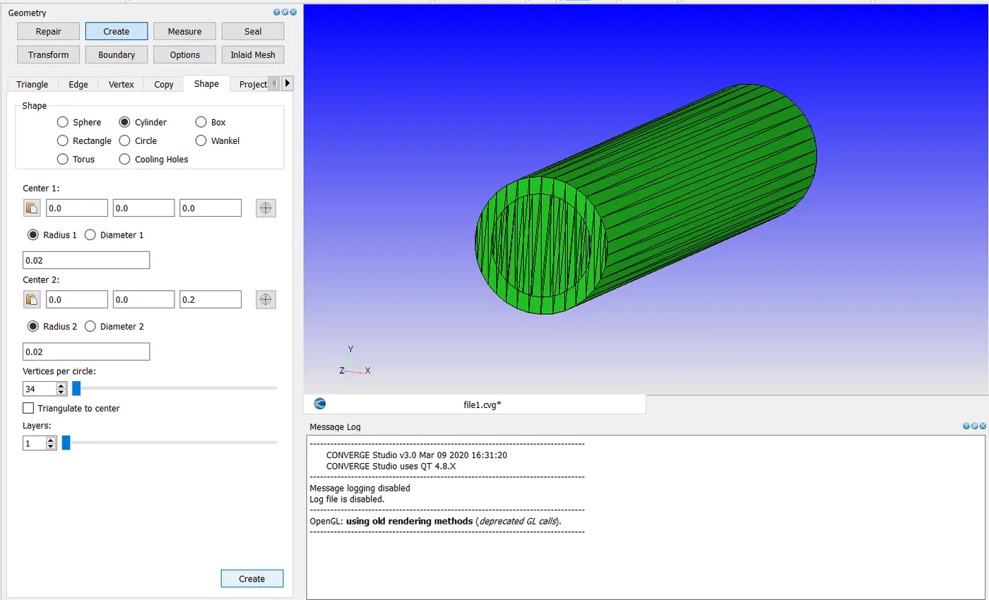
Then For creating pipe shaped geomentry Add the thickeness as shown.
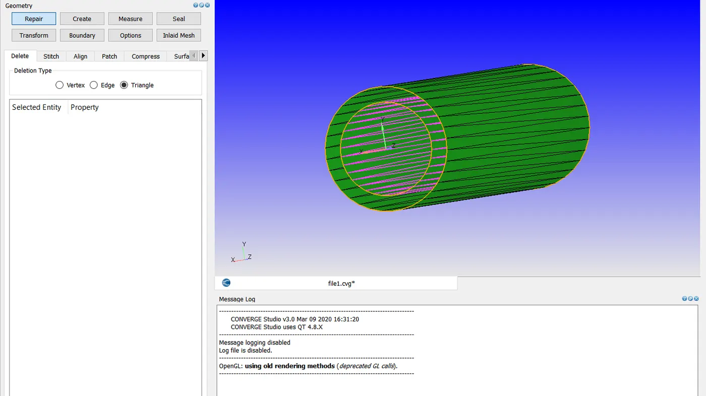
deleting the Front and back thickness wall by using repair tools.
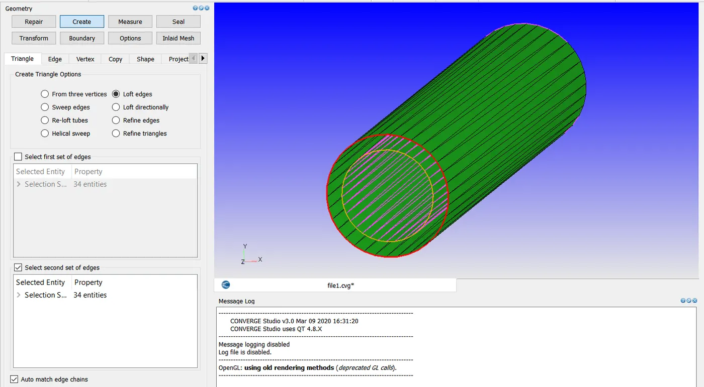
By using create loft edges The thickness of pipe is added.
This is the goementry after adding thickness.
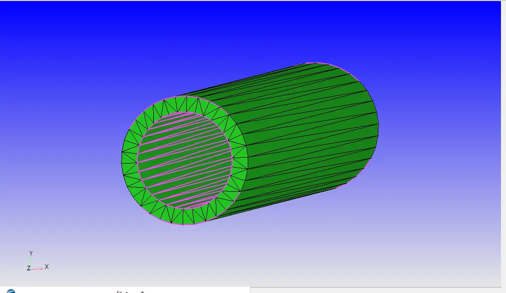
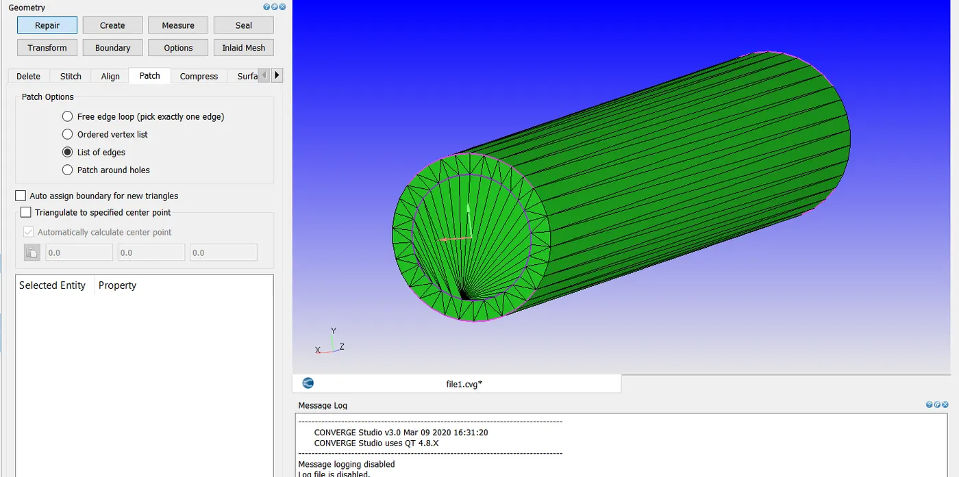
Finally for inlet and outlet specification patch the both sides as shown in fig.
Step:2:
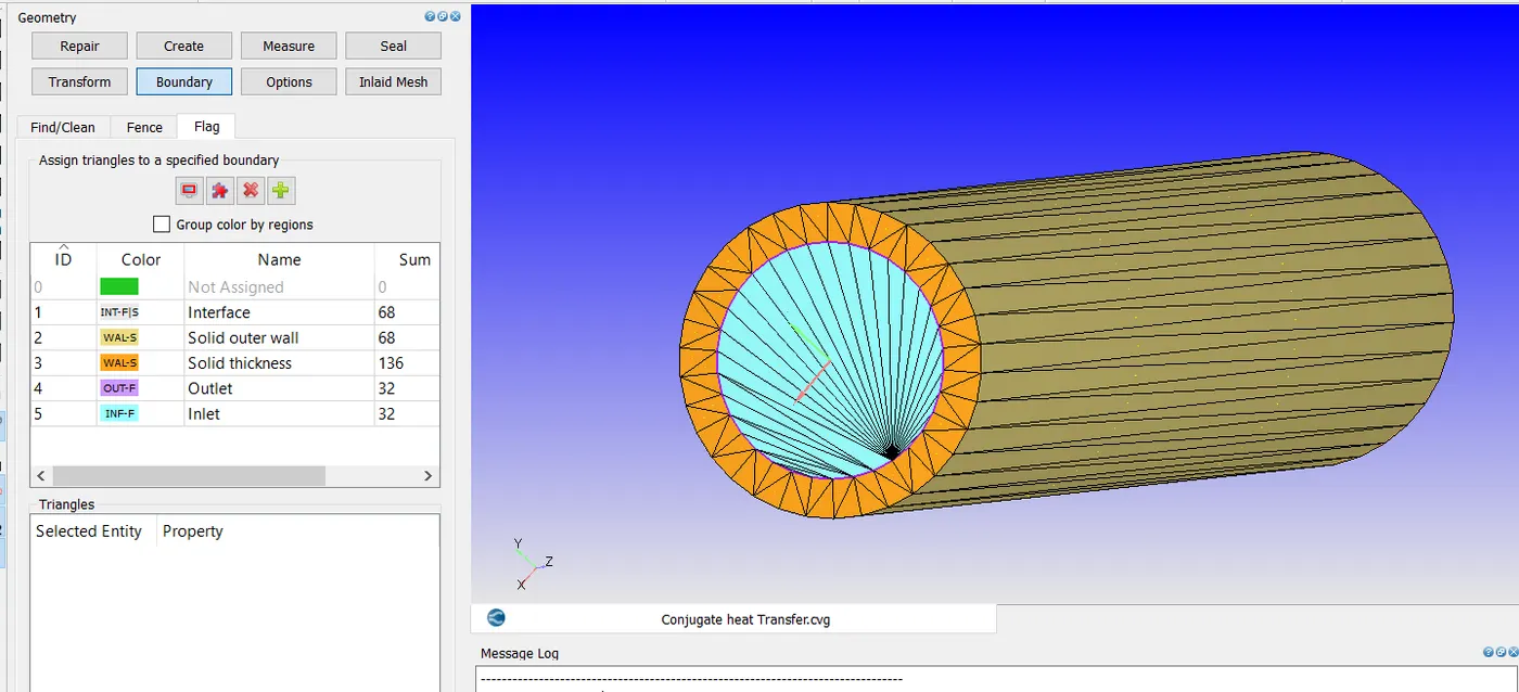
In this step, we take triangular structures and flag them together as boundaries which are marked with different colours. This is done so that the boundary conditions can be assigned to each triangular structure.
Giving boundaries by selecting the sides which can help with other steps for simulation.
Once the boundaries have been flagged, we assign the different boundary conditions for the flow to take place within the geometry.
Step:3:
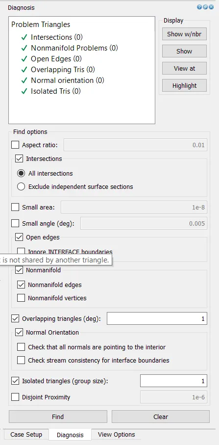
Check whether there is any errors by using diagnosis tool as shown below.
Step:4:
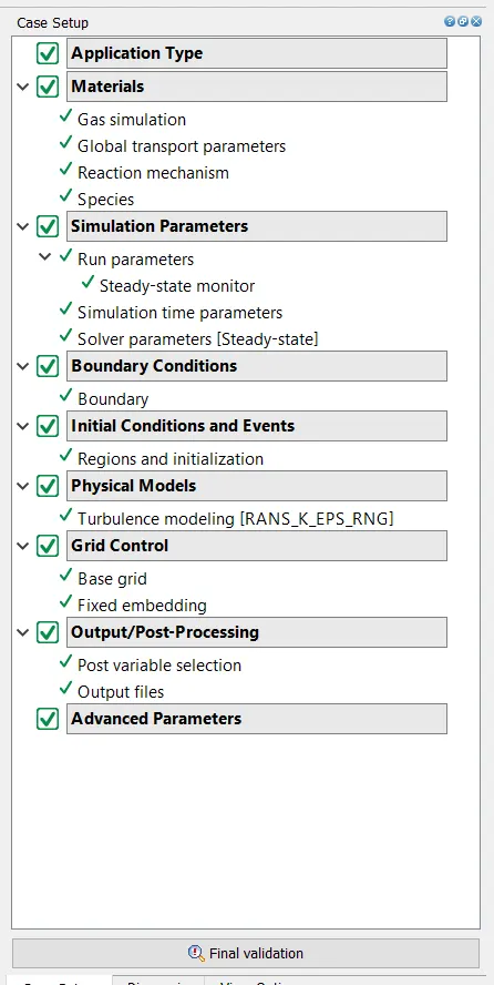
These are the following steps for setting up simulation for Backward facing step.
Step:5:
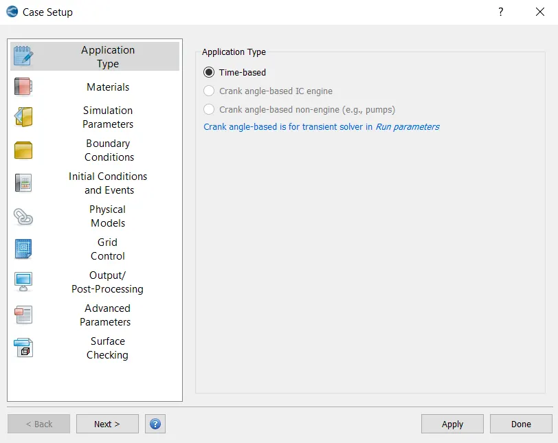
Select the application type time based for steady state simulation.
Step:6:
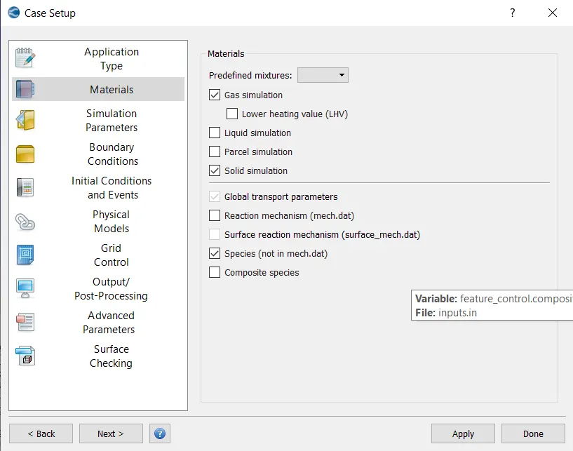
Select the material type for the flow through geomentry .here Air is the material taken.and aslo this simulation includes both fluid and solid simulation. so select solid simulation check box and also unselect the reaction mechanism.
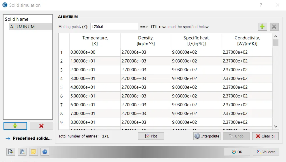
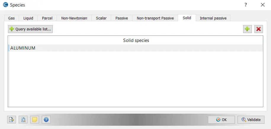
Adding the solid material for simulation in solid simulation box.
Adding both fluid and solid species for simulation.
Step:7
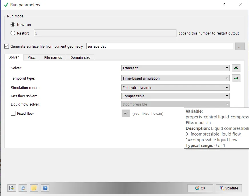
Select transient solver for the simulation.
Step:8:
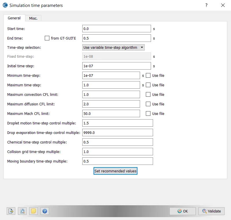
Here we can define the start and end time for The simulation
and also the initial and minimum time step.
Step:9:
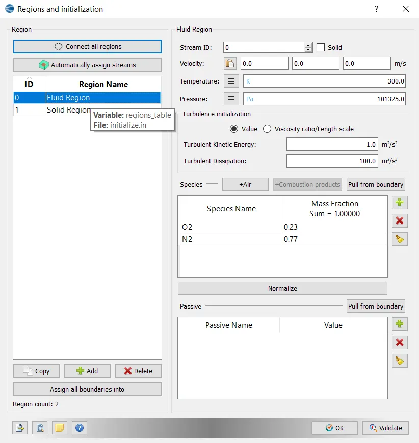
The boundaries are to bounded to a region for the steady simulation.so that volumetric region are created with the species of air.
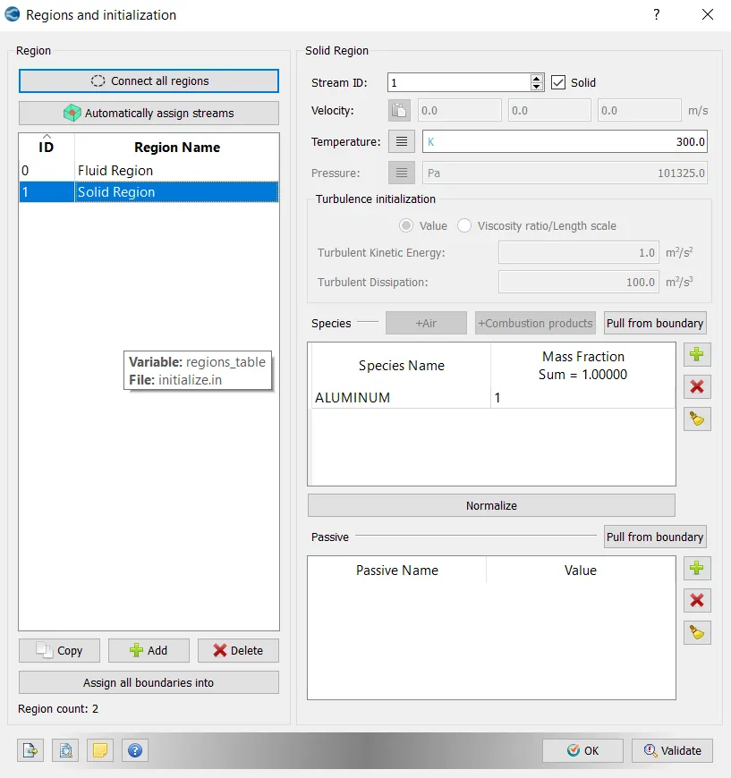
There are two regions in this simulation. One is Fluid region (Stream ID = 0) and it is added with species as Air. The second region is solid with stream ID = 1 and the solid check box is checked. The solid species is Aluminum.
Region for Fluid :
Region for Solid:
Step:10:
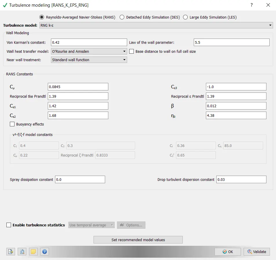
Here select the turbulance model that can be used for simulation.
Step:11:
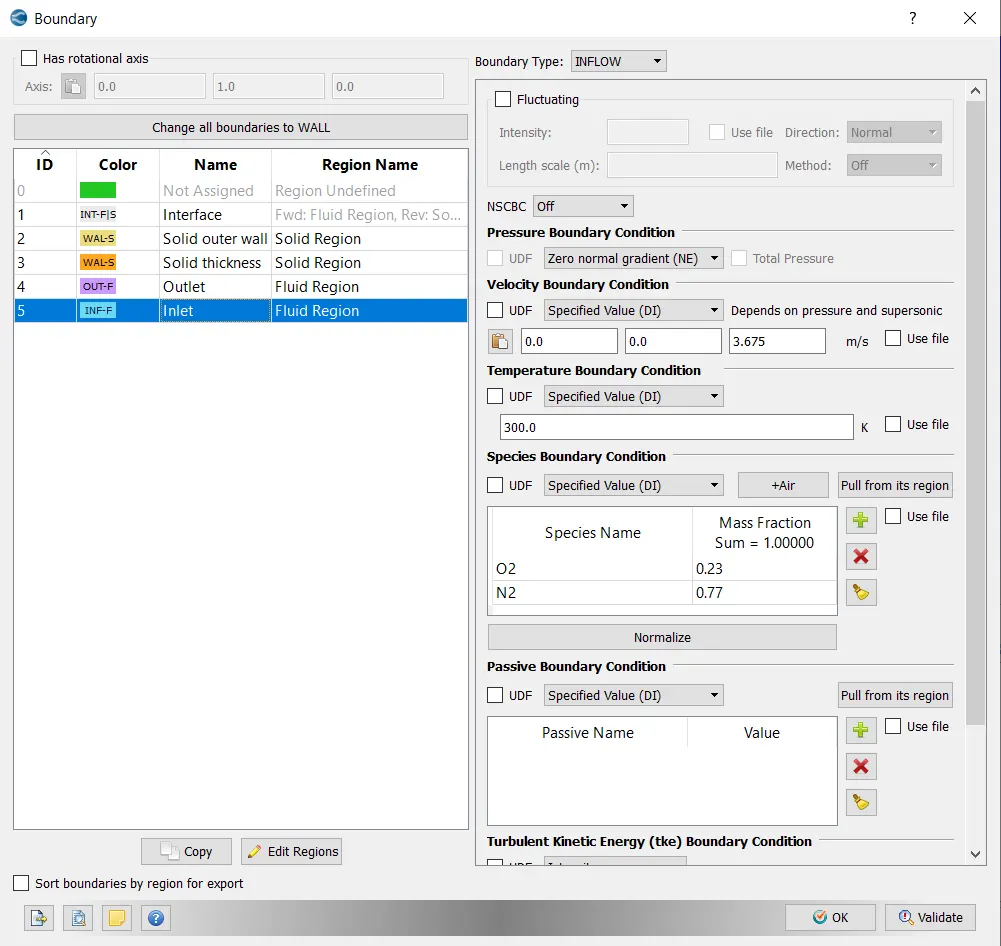
In here the boundary conditions are given to the volumetric regions and also the inlet conditions are given .
pressure and temperature are defined for inlet.
Inlet:
In Inlet the velocity is calculated based on given Inlet Reynolds number = 7,000
By using formula
Re = (rho*V*D)/(Dynamic viscosity)
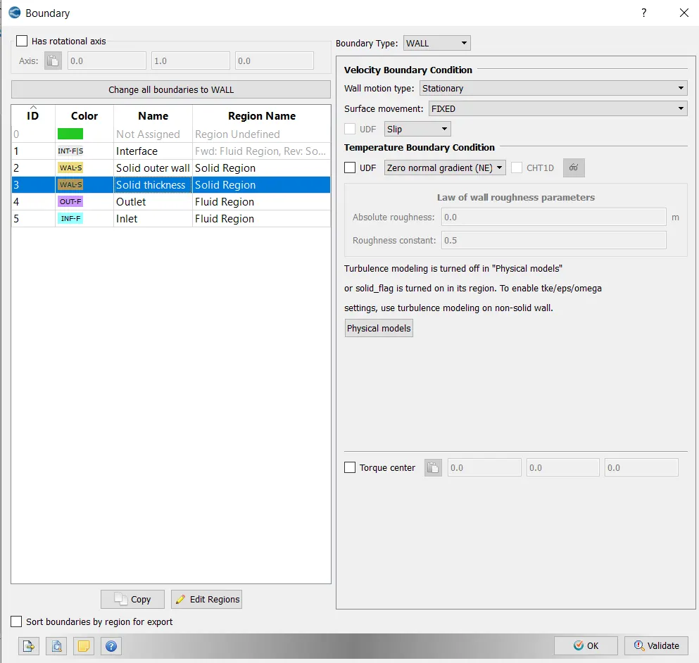
Solid thickness:
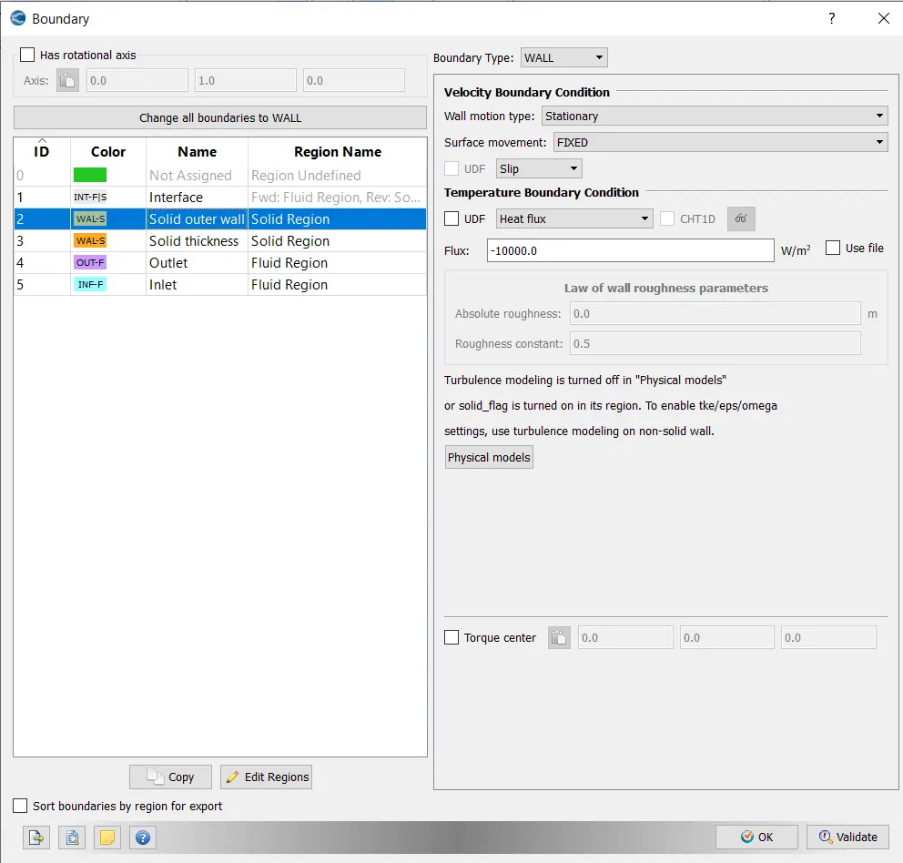
Solid outer Walls:
In here walls are defined to slip and heat flux value is specified.
Interface:
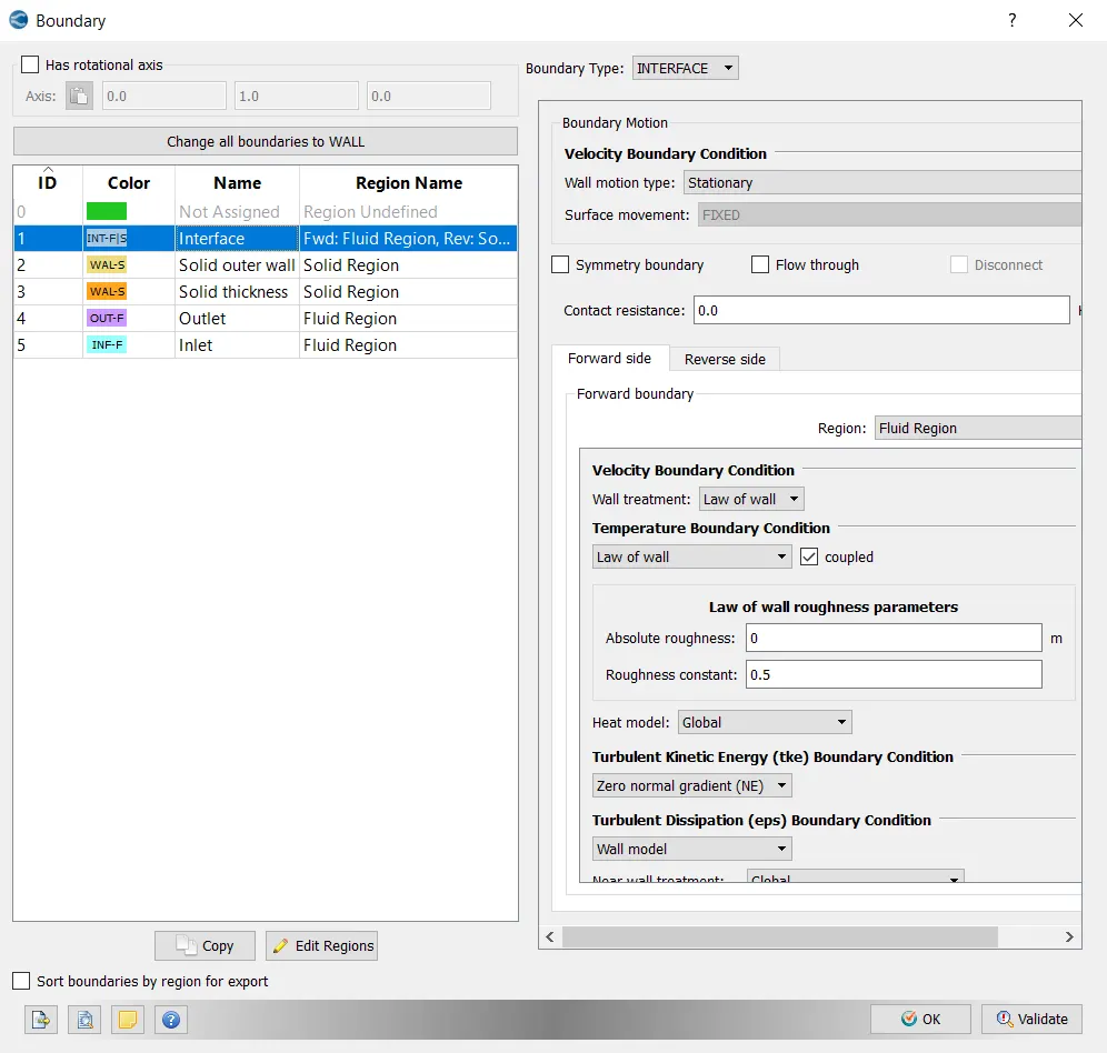
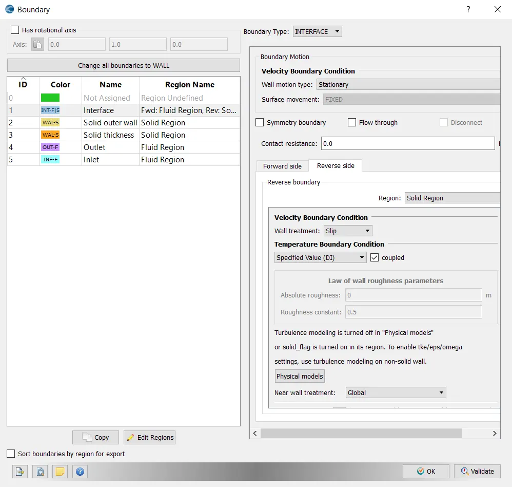
Inner Wall is the Interface between Solid and the Fluid. Therefore it is an INTERFACE Boundary. The forward boundary is Fluid Region with Law of Wall and the reverse boundary is the Solid Region with Slip Wall.
For Fluid region
For solid region:
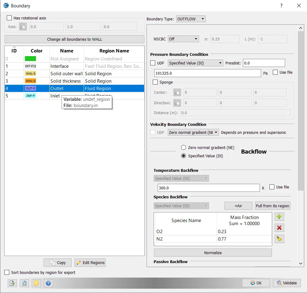
Outlet:
here the outlet pressure value is specified
species used for simulation is defined in outlet.
Step:12:
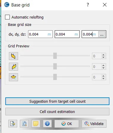
The basic mesh size of the Geomentry is specified here.
Step:13:
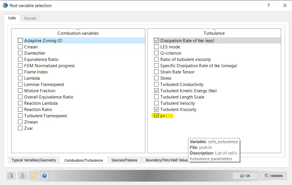
In post variable selection turn on the Y plus check box so that we can analyze in paraview.
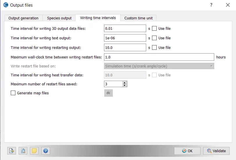
in output files the time interval for 3D output and text output is specified.
Step:14:
Finally the specified case setup file are exported to folder and run simulation.
The simulation for number of cycles are run in cygwin command window.
Step:15:
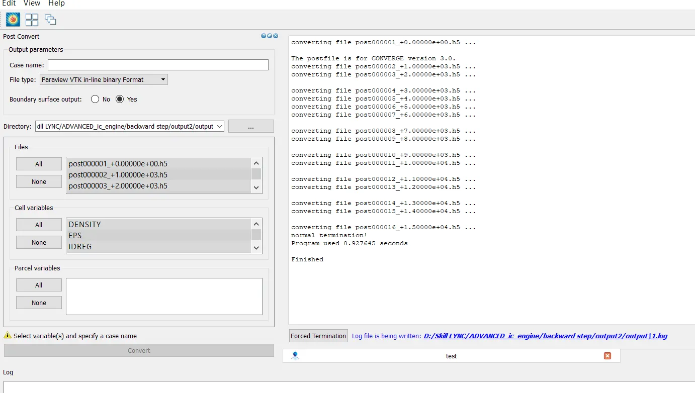
Post convert the files that is simulated in cygwin command window and file name is given .
Step:16:
Software used: ParaView As the simulation is binary files called “post” files are generated inside the output folder. These files have an extension *.out. Now these files are written by CONVERGE. These files contain information regarding the 3D flow field. We use a special software called ParaView that can read this flow information. However, before ParaView can do this, the files have to be converted to a form that ParaView can understand. This is done using a tool called post convert. After the conversion, we load the files into ParaView.
SIGNIFICANCE OF Y+ IN K-EPSILON TURBULENCE MODELLING:
y+ is a non-dimensional distance. It is often used to describe how coarse or fine a mesh is for a particular flow pattern.
It is important in turbulence modeling to determine the proper size of the cells near domain walls.
The turbulence model wall laws have restrictions on the y+ value at the wall.
A non-dimensional wall distance for a wall-bounded flow can be defined in the following way:
Where, U* is the friction velocity at the nearest wall,
y is the distance to the nearest wall and
v is the local kinematic viscosity of the fluid.
Results:
Grid Independence Test.
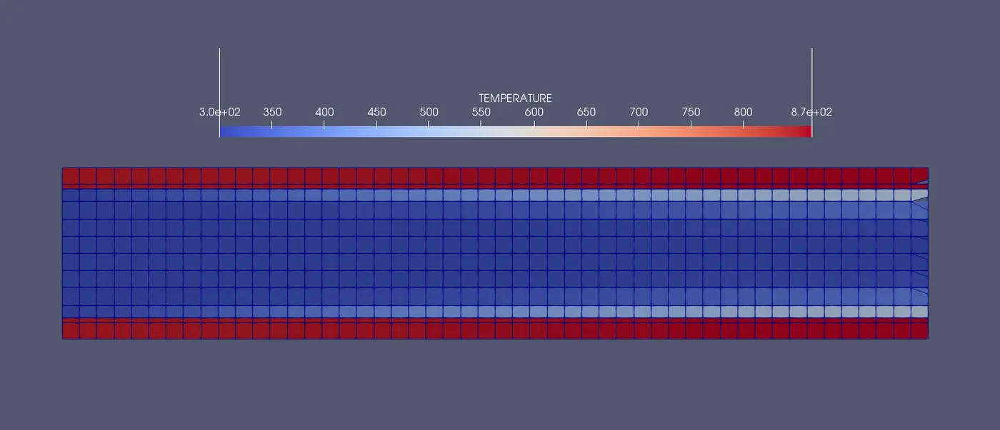
Case:1
Base grid size: 0.004 m
Mesh:
Temperature Contour:
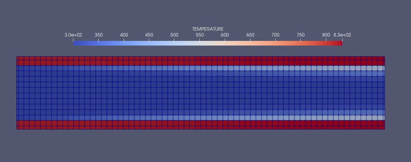
Case:2
Base grid size: 0.003m
Mesh:
Temperature Contour:
Case:3
Base grid size: 0.002 m
Mesh:
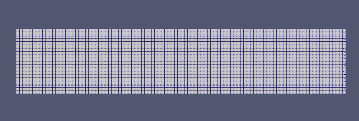
Temperature Contour:
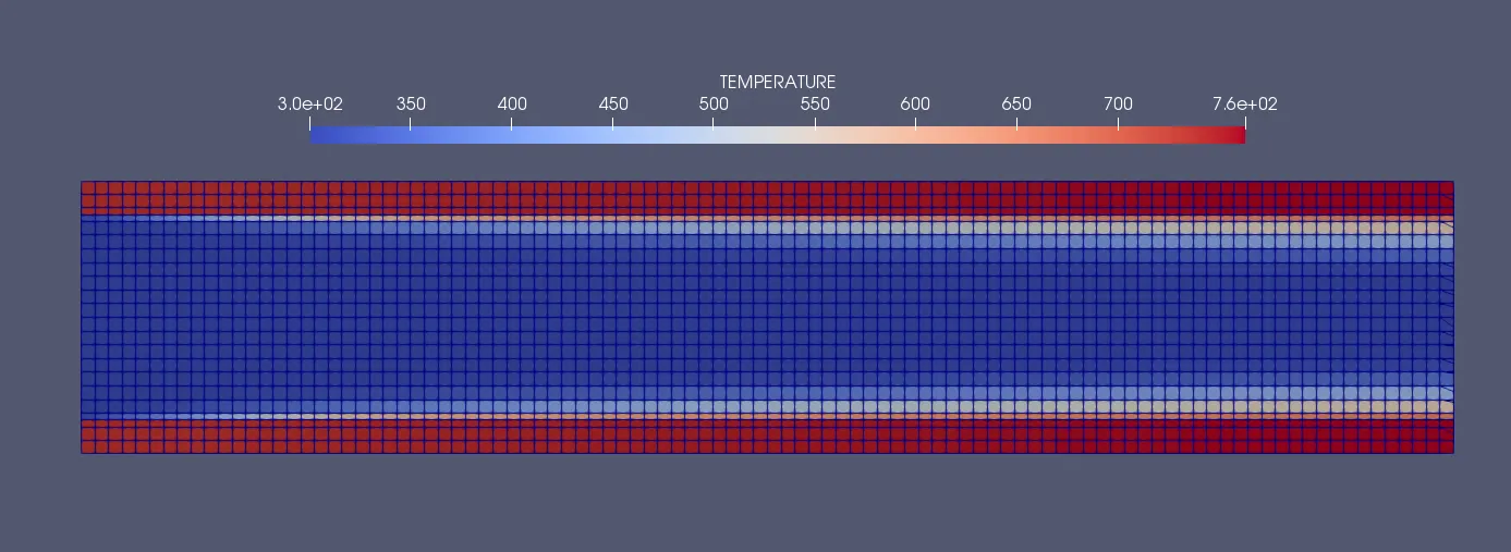
Comparison of Three Cases:
Plot:
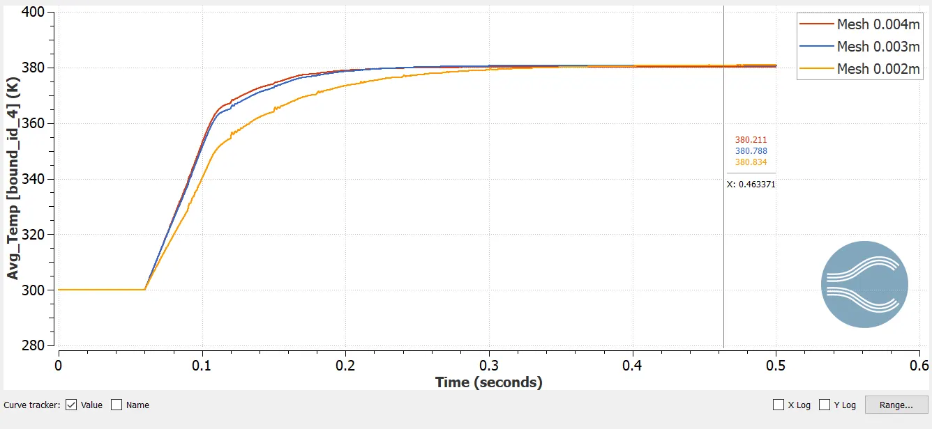
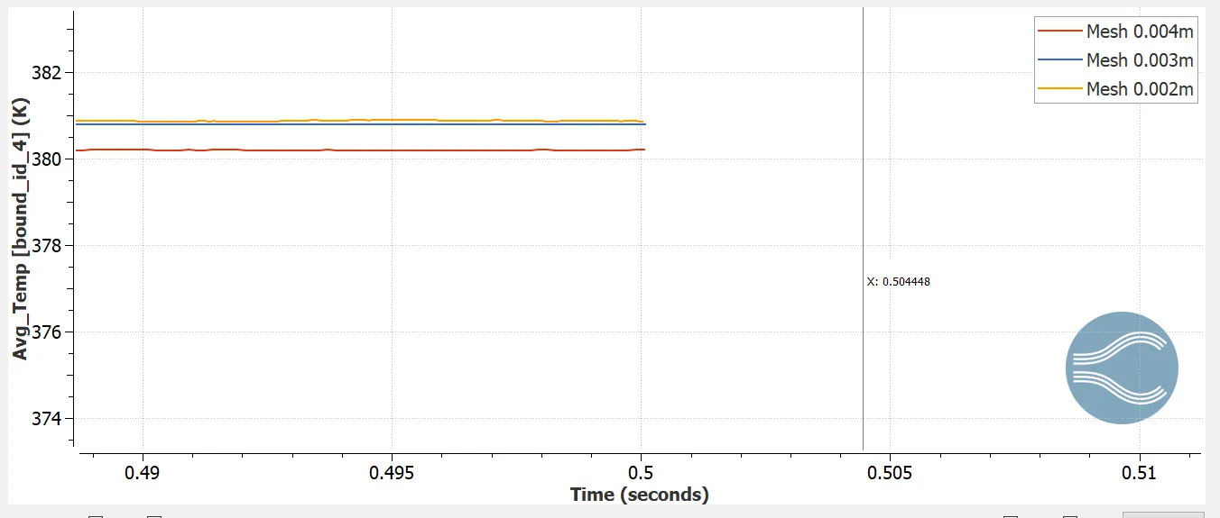
From the above contours and the mean temperature (vs) time graph it can be seen that the outlet mean temperature does not converges at the same value for all the three grid sizes. The convergence of outlet mean temperature for the grid size 2 mm is good.
It reaches the steady state gradually for 2 mm grid size. Here the grid size of 2mm passes the grid dependence test. But further reducing the grid size to 1 mm can give more accurate results and it requires more advanced computers.
Hence the grid dependence test is carried out for selecting the optimum grid size for the best convergence of the results.
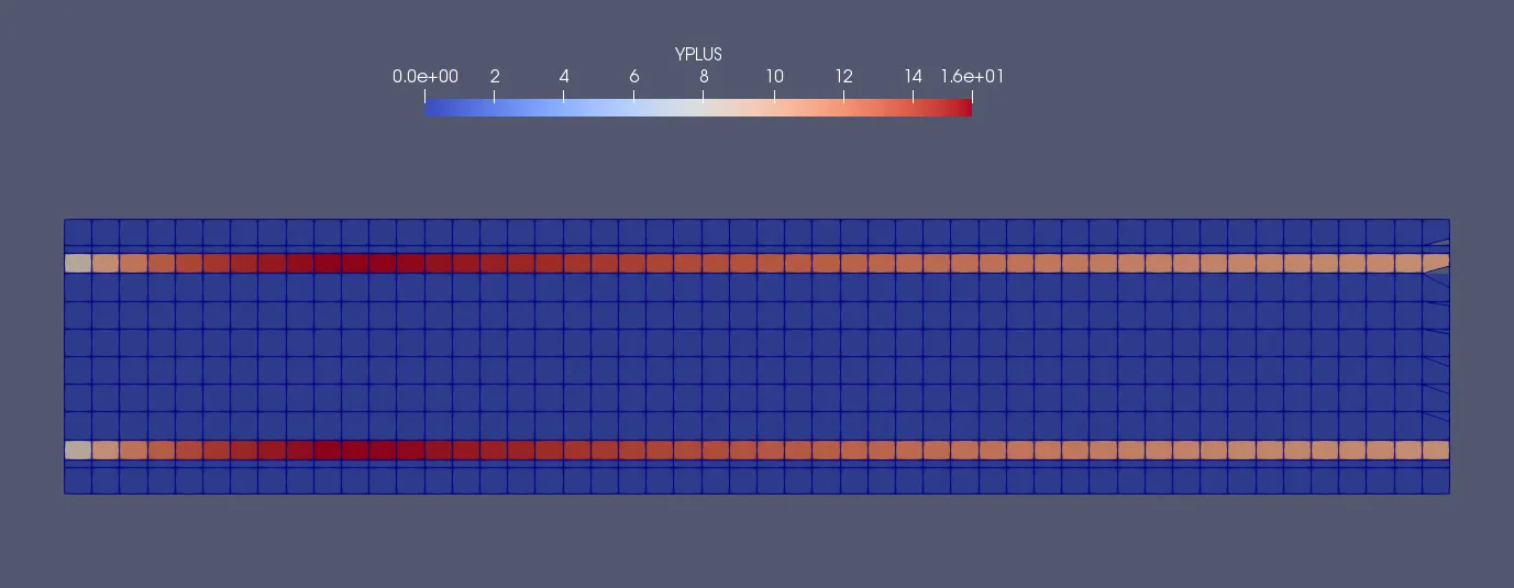
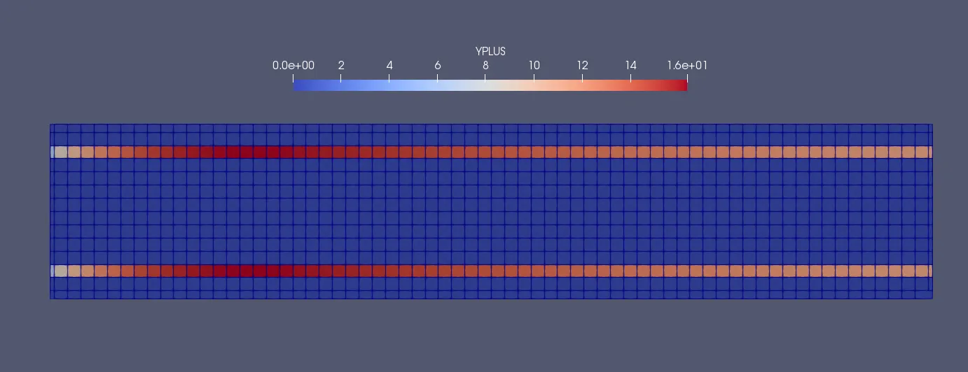
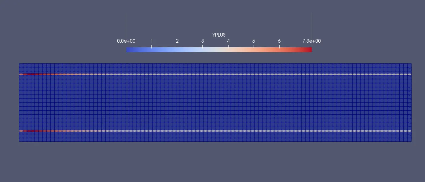
y+ VALUE:
The y+ value is a non-dimensional distance (based on local cell fluid velocity) from the wall to the first mesh node.
The main benefit of this wall function approach lies in the significant reduction in mesh resolution and thus reduction in simulation time.
For flows where wall-bounded effects are not a priority, or if separation is expected to occur only due to sharp changes in the geometry, an ε-based wall function approach is more than sufficient. One of the reasons for the need of y+ is to distinguish different regions near the wall or in the viscous region.
Near-wall regions have larger gradients in the solution variables, and momentum and other scalar transports occur most vigorously. The wall distance y+ is a non-dimensional distance similar to local Reynolds number, often used in CFD to describe how coarse or fine a mesh is for a particular flow. It is the ratio between the turbulent and laminar influences in a cell.
Very close to the wall, viscous damping reduces the tangential velocity fluctuations, while kinematic blocking reduces the normal fluctuations.
Towards the outer part of the near-wall region, however, the turbulence is rapidly augmented by the production of turbulent kinetic energy due to the large gradients in mean velocity.
Accurate presentation of the flow in the near-wall region determines successful prediction of wall-bounded turbulent flows.
The k-ε models are primarily valid for turbulent core flows (i.e., regions somewhat far from walls) and hence are coupled with wall functions to bridge them with the solution variables in the viscosity-affected region.
The use of wall functions for these class of flows should be avoided as their use will limit the overall number of mesh nodes that can be sensibly placed within the boundary layer.
Grid Size: 4mm:
Grid Size: 3mm:
Grid Size: 2mm:
Very close to the wall, viscous damping reduces the tangential velocity fluctuations, while kinematic blocking reduces the normal fluctuations.
Towards the outer part of the near-wall region, however, the turbulence is rapidly augmented by the production of turbulent kinetic energy due to the large gradients in mean velocity.
Accurate presentation of the flow in the near-wall region determines successful prediction of wall-bounded turbulent flows.
The k-ε models are primarily valid for turbulent core flows (i.e., regions somewhat far from walls) and hence are coupled with wall functions to bridge them with the solution variables in the viscosity-affected region.
The use of wall functions for these class of flows should be avoided as their use will limit the overall number of mesh nodes that can be sensibly placed within the boundary layer.
EFFECT OF SUPERCYCLING STAGE INTERVAL
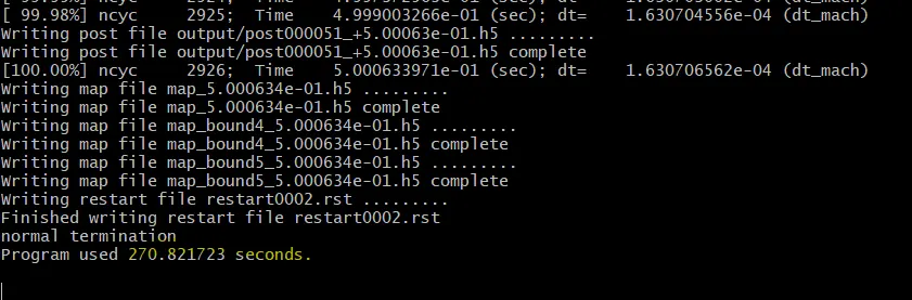
For SSI 0.03:
For SSI 0.02:
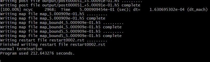
For SSI 0.01:
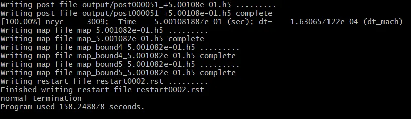
The solution Time decreses as we decrease the SSI values As above shown figures.
Increasing the SSI for the simulation does not mean that it will reduce the total simulation time as in the case of base grid. The simulation time is based on the number of transport and other equation to be solved and on the grid size.
Here this occurs because, the studio has to transfer the information from one stage to the other and sometimes this information can be huge. By optimizing the values, the computational time will become dependent on the stage intervals.
The supercycling stage intervals does not have any significant effect on the final temperature values.
CONCLUSION:
From this conjugate heat transfer simulation, one can understand that it is the transfer of heat occurring simultaneously between the solid and fluid regions.
In this simulation, the fluid part is solved using Navier-Stokes and energy equations and the solid part is solid using the solid heat equation.
The importance of y+ value while solving the wall bounded problem is also understood. The technique of supercycling is used here.
The supercycling method first solves the fluid part and the solid interface part together. Then it makes the results as the boundary condition at the interface to solve the solid part as a steady state by freezing the fluid solver.
Then the solid temperature is updated and the fluid part in unfreezed. This cycle takes place till the solid temperature converges.
The conjugate heat transfer simulation is used for efficiently combining heat transfer in fluids and solids for designing effective coolers, heaters, or heat exchangers.
Heat transfer in fluids and solids can also be combined to minimize heat losses in various devices.