Week 6: Conjugate Heat Transfer Simulation
Aim :
To Setup a flow simulation through a pipe with a thickness of 5mm having an Inlet Reynolds number of 7,000.
To perform grid independency test and show that the outlet temperature converges to a particular value.
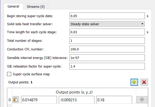
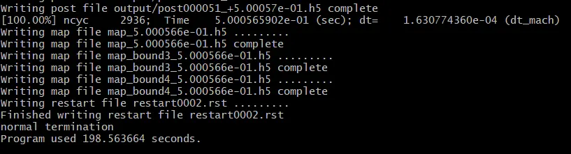
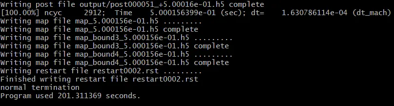
To Set supercyle stage interval to 0.01,0.02 and 0.03 and see how the total simulation time compare against the baseline configuration.
Introduction & Geometry :
To calculate a heat transfer analysis, we must have two phases where the heat is transfered between.
Thus the pipe through which air flows is taken with a thickness and the solid material used for the pipe is alumium.
The inner radius (Fluid Radius) is 0.015 m and the Outer radius is 0.020 m. The length of the cylinder is taken as 1m.
Now we can name different surfaces of the pipe to our convinience.
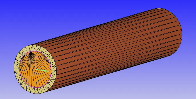
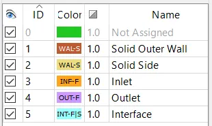
The surface seperating the solid and the fluid region is named as the interface.
Case Setup :
The Simulation can be carried out on a time based calculation.
In the materials window select solid simulation & species as we are using solid material for the pipe in the simulation.
Select air as the fluid medium and aluminium as the solid medium. Choose the solid material as aluminium in the species windpw and add O2 & N2 for fluid medium.
In the simulation parameters, use the transient simulation type for compressible fluids. Specify the end time of the simulation to be 0.5 seconds.
Boundary Conditions :
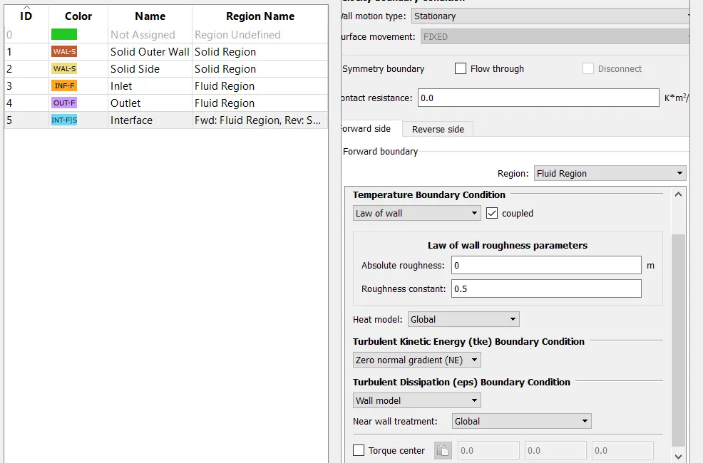
The outer solid wall of the pipe is assumed to be exposed to a heat source. Thus the boundary conditions are given as slip wall with a flux value of -10000 W/m^2 around the pipe.
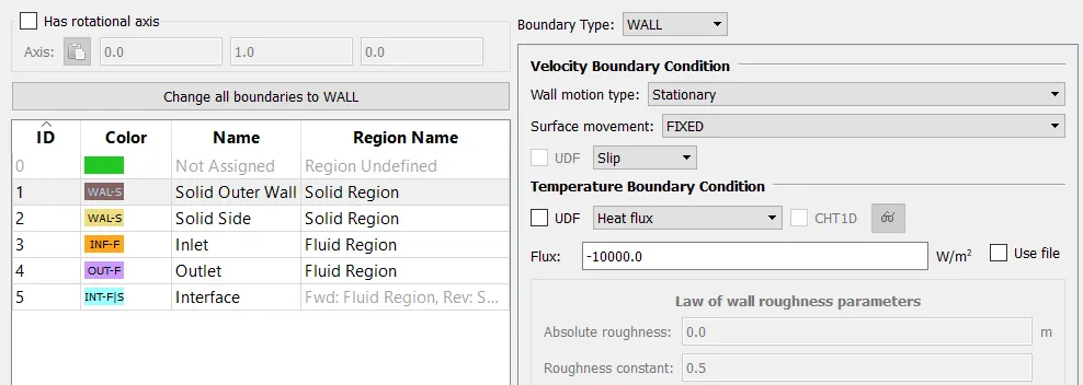
The Solid sides (Thickness) of the pipe are also set to wall with slip conditions.
The inlet boundary conditions is set to inflow, Where the velocity is specified. The inlet velocity is calculated by the given reynold's number.
Re = (rho*V*D)/(Dynamic viscosity)
Re*(Dynamic viscosity)/rho*D= V
Re = 7000; Dynamic viscosity = 1.853 e-5 kg/ms ; rho = 1.176 kg/m^3; D = 0.03m
Thus V = (7000*1.853e-5)/(1.176*0.03)
V = 3.675 m/s.
Thus the inlet velocity is calculated as 3.675 m/s which is substituted in the Z direction of the inlet conditions as the length of the pipe is along the Z direction.
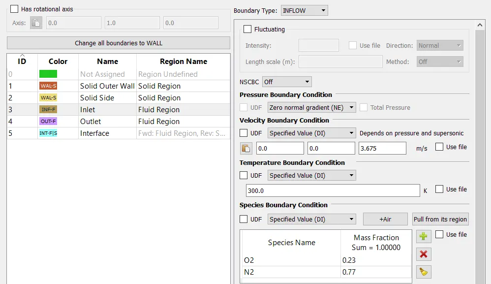
The outlet conditions are set to outflow and the pressure outlet is set to atmospheric pressure of 101325 pa.
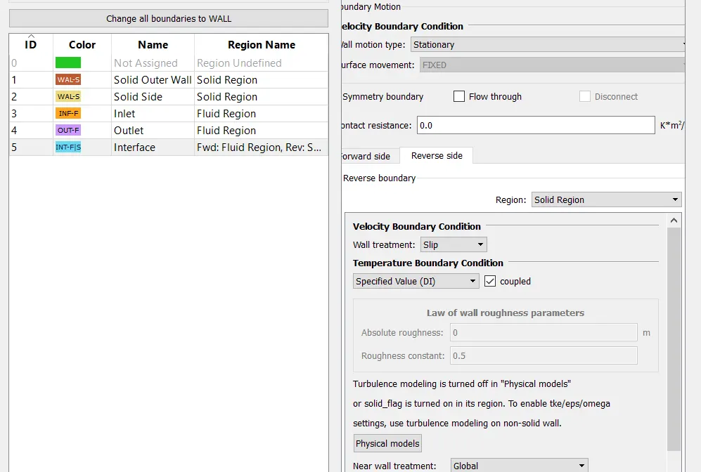
The interface boundary condition has a forward side to be fluid and the backward side to be solid region. Both the conditions are specified to the interface window.
Region & Initialisation :
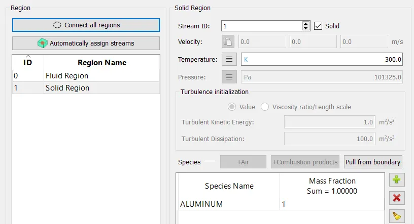
The fluid region is specified and updated with air as the material and the default initial conditions for pressure and temperature properties.
The solid region has to be specified seperatly with a stream ID of 1 and the material as aluminium.
Physical Models :
In the physical models use the default K-Eppsilon model as the turbulence model.
Also Use the super cycling to speed up the simulation time.
Grid Control :
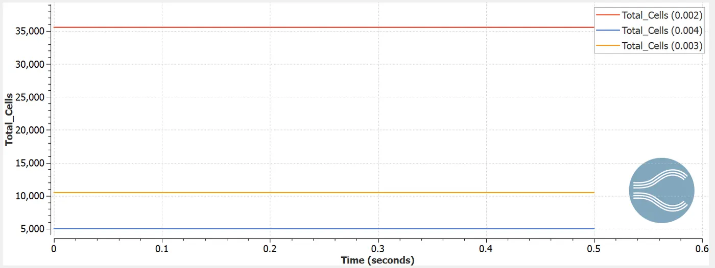
Here we are going to use three different grid size for doing the grid independency test.
The grid sizes are refined to see the changes in the output properties.
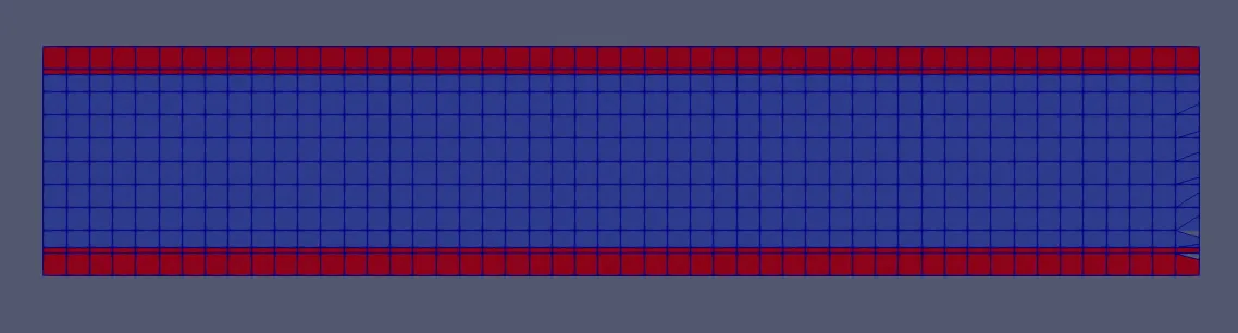
The grid sizes are taken to be 0.004;0.003;0.002 m.
0.004 m :
0.003 m :
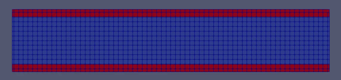
0.002 m :
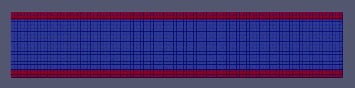
Post processing :
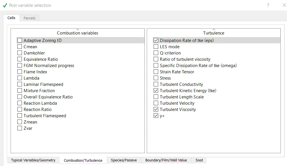
Activate the y+ monitor in the post processing controls to calculate the y+ values for further evaluation.
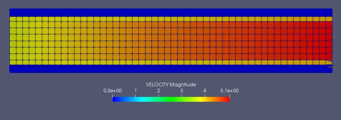
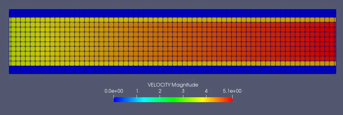
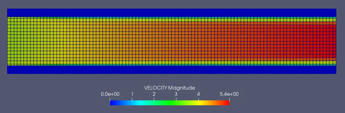
Velocity contours :
0.004 m :
0.003 m :
0.002 m :
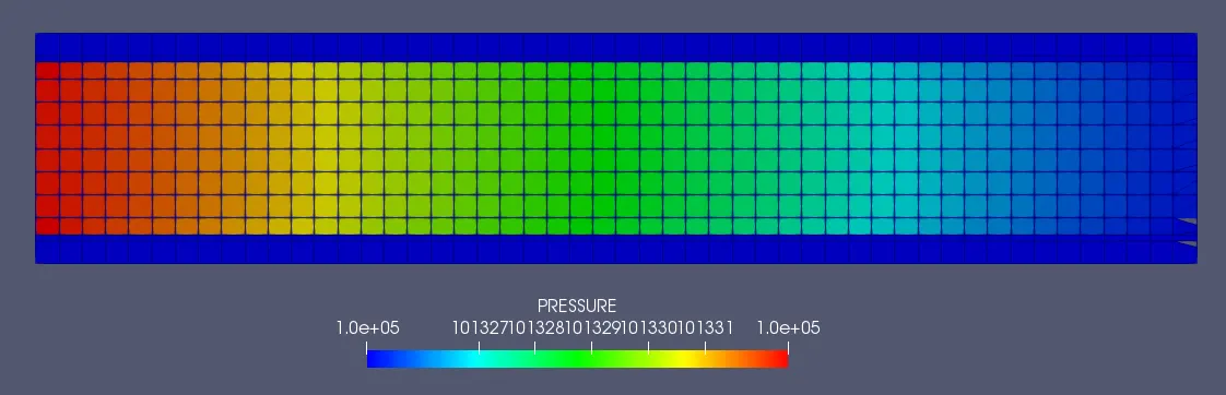
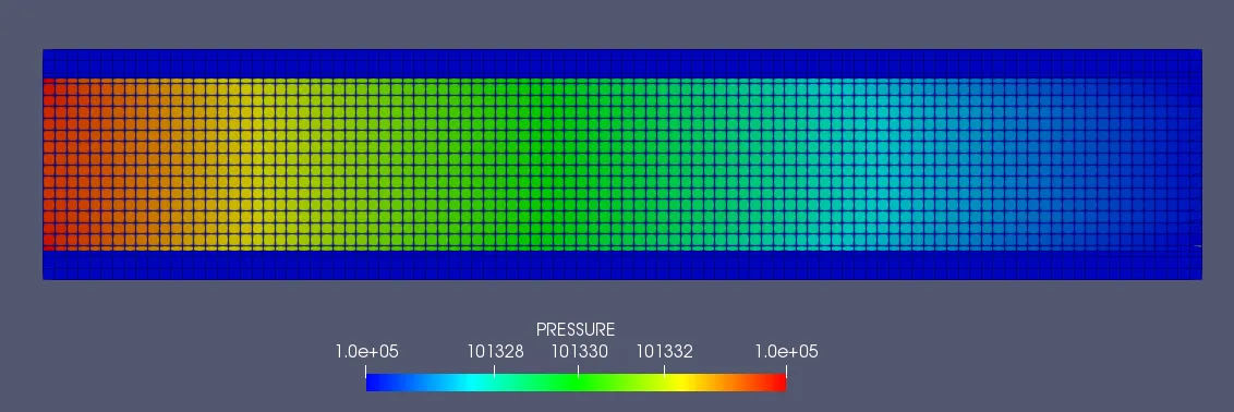
Pressure contours :
0.004 m :
0.003 m :
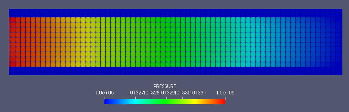
0.002 m :
Temperature contours :
0.004 m :
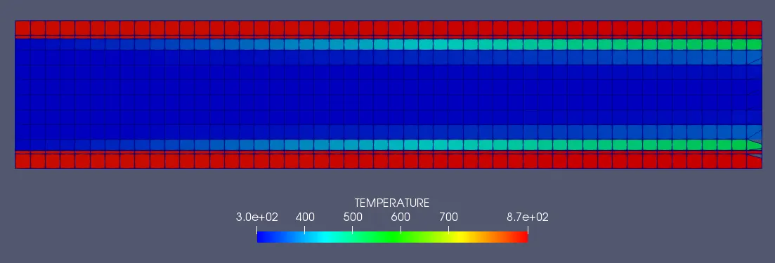
0.003 m :
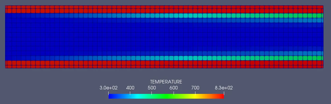
0.002 m :
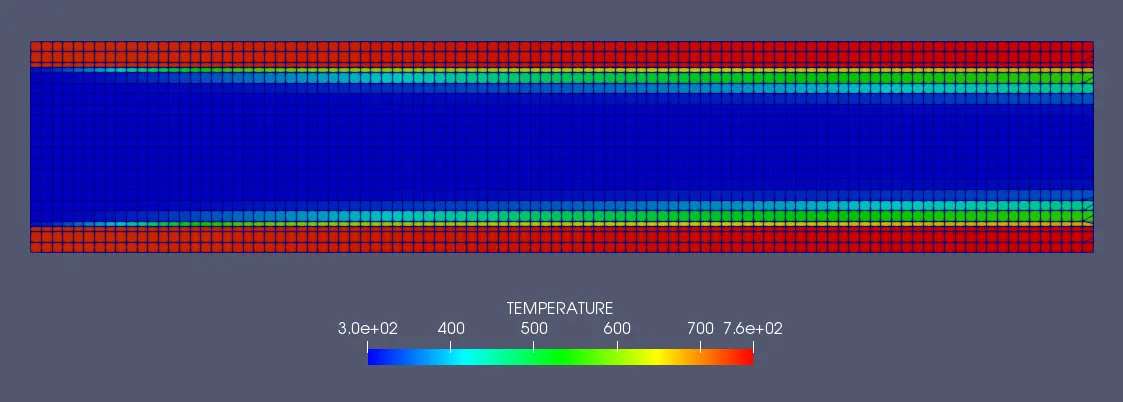
Conclusion on Contours :
The contours are observed for different refined meshes. We can see some changes in the properties of the flow as the mesh gets refined.
The velocity of the fluid flow enters the inlet and as it moves it loses the velocity near the walls of the pipe due to friction and the velocity at the center of the pipe gets increased.
The temperature around the pipe exterior walls gets transfered through the solid pipe to the fluid flowing inside the pipe. As the flux around the pipe reaches the pipe the solid surface absorbs the heat due to conduction and transfers the heat to the fluid through convection. We can see that the temperature of the air near the walls of the pipe is higher than at the center.
As the mesh gets refined we can see more accurate changes in the temperature near the walls of the pipe.
Grid Independency Test :
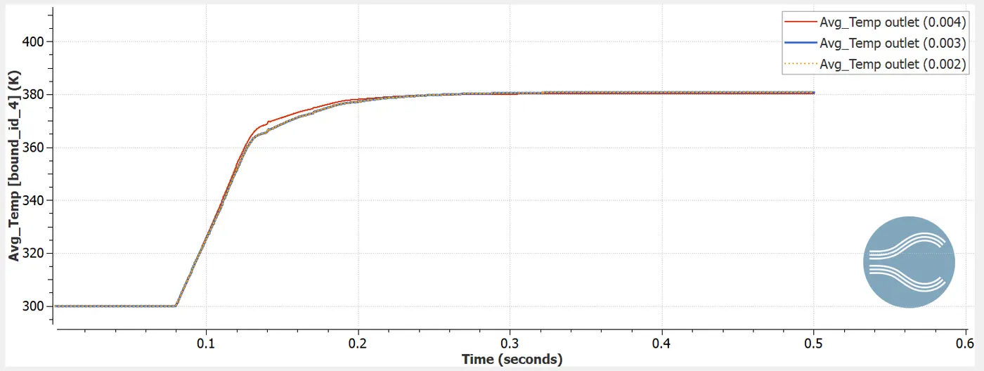
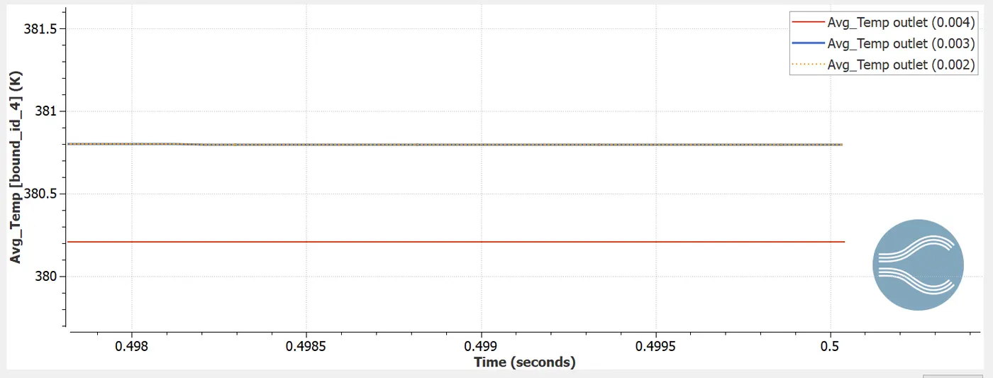
Here we can see the temperature plot of area average temperature at the outlet end of the pipe.
We know that the outlet area is subjected only to the fluid particles. Thus the outlet average temperature calculates the average temperatures of the air at the outlet phase.
As we can see that the temperature after convergence chenges for refined meshing.
The temperature average for the base mesh is different than the temperature average of the other two refined meshing.
As the temperatures of the refined meshes are converged to the same value, we can say that the simulation is independent of grids after the refinement.
Y + :
0.004 m :
0.003 m :
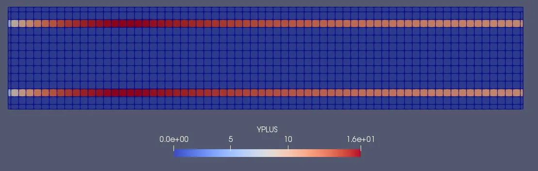
0.002 m :
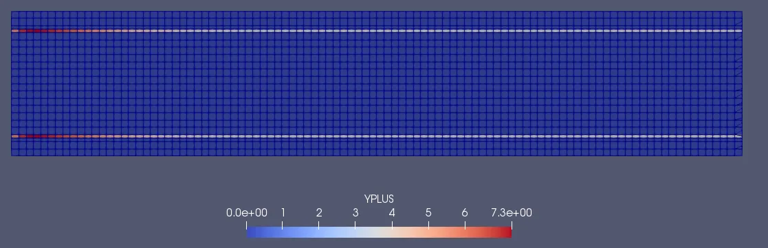
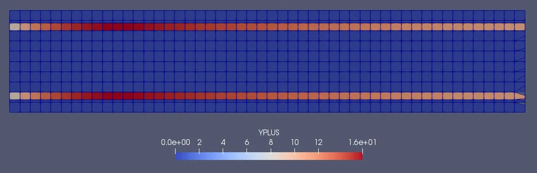
The y+ value is a non-dimensional distance (based on local cell fluid velocity) from the wall to the first mesh node, as you can see in the image below.
We can see that as the mesh gets refined, we get more accurate y+ values for the flow.
The y+ value is more near the inlet. It increases as it starts the flow and gradually starts to decrease and converge as it travels towards the outlet.
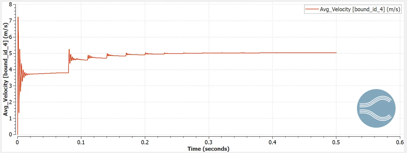
Velocity Plot :
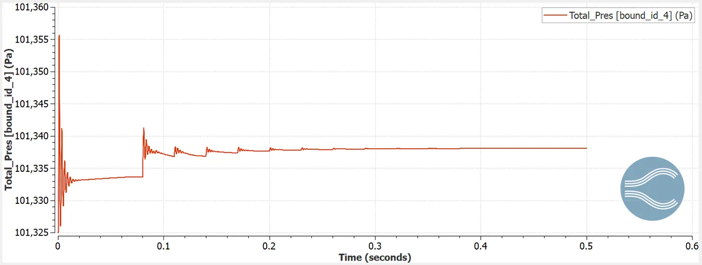
Pressure Plot :
Cell count :
Super Cycling Time Intervel :
0.01 :
0.02 :
0.03 :
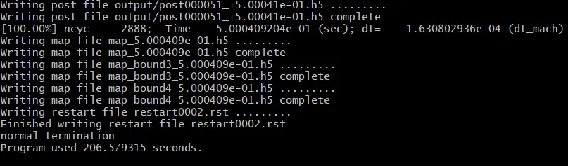
As the super cycling intervel is reduced, The simulation time also gets reduced.
As the calculation of the flow attains a much lesser intervel size, the calculation becomes faster as it takes the values and progress for a shorter intervel.
As we increase the intervel size the time to attain steady state also increases which in return increases the simulation time.