Week 6: Conjugate Heat Transfer Simulation
Aim: To perform Conjugate Heat Transfer Simulation in converge software.
Theory:
Conjugate heat transfer:
Conjuate Heat Transfer is combination of heat transfer in solid and heat transfer in fluid.
In solid, conduction often domain whereas in fluid convection usually domain.
Conjugate heat transfer is observed in many situation. For egs, heat sinks are optimized to combined heat transfer by conduction in the heat sink with the convection in the surrounding field.
Inlet Reynolds number should be 7,000
Super cycling:
This method is used by converge in CHT problems involving both solid as well as fluid regions.
Since solving in the fluid domain is much faster due to the time scale difference for heat transfer in liquids comapred to solids.
The solid state solver might not have reached the steady state in the time liquid solver does.
So in supercycling the fluid domain solver is paused until the solver for solid domain converges. This pausing is done in intervals and is user defined.
Re = (rho*V*D)/(Dynamic viscosity)
rho = 1.225 kg/m3
V to be calculated
D = 0.015 m.
Dynamic viscosity = 18.45 * 10-6">10^−6 Pa.s
v = 7.028 m/s
Simulation Procedure:
Geometry Modelling:
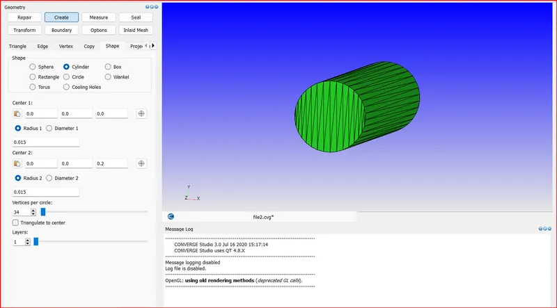
Create a cylinder with the following dimensions.
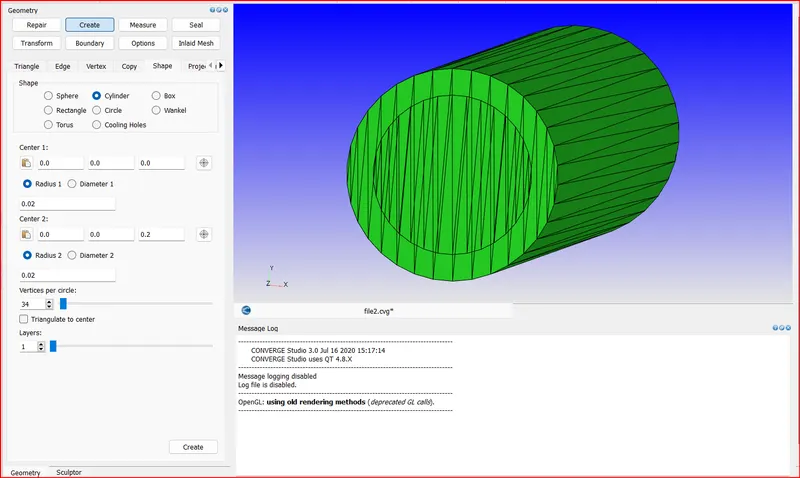
Add thickness to the above cylinder.
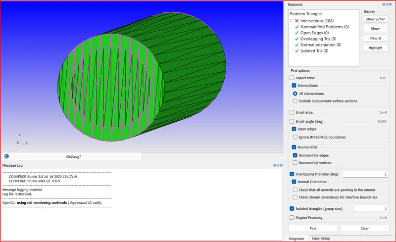
On running the diagnosis check we can see that intersection errors are appearing.
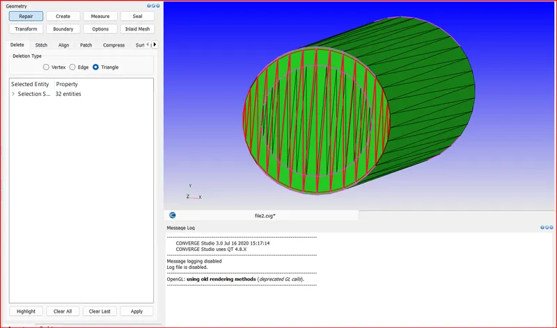
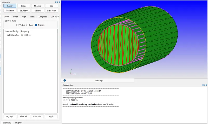
To eliminate and repair the errors, first delete the highlighted faces.
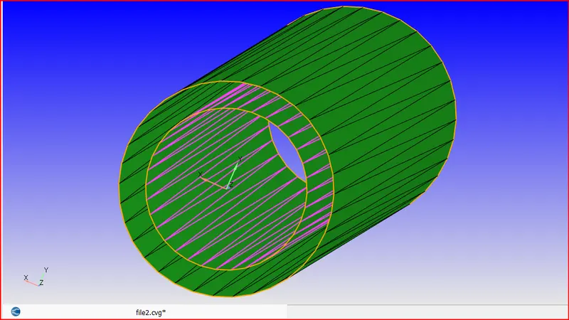
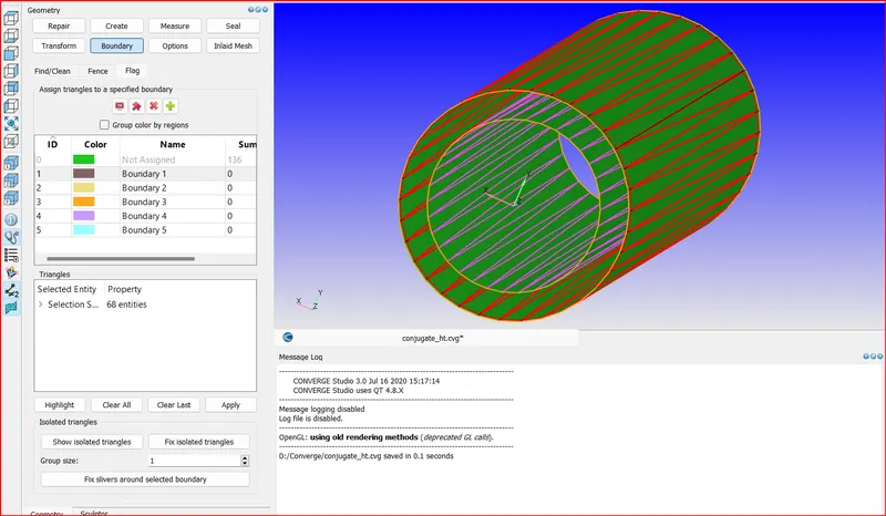
Now create and assign the boundaries.
Go to create> traiangle> Loft edges> by open edges and select the two set of open edges. to create a face.
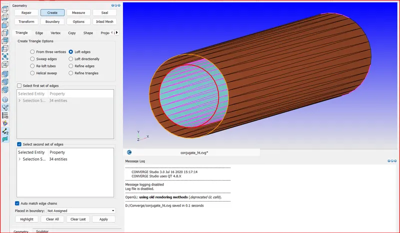
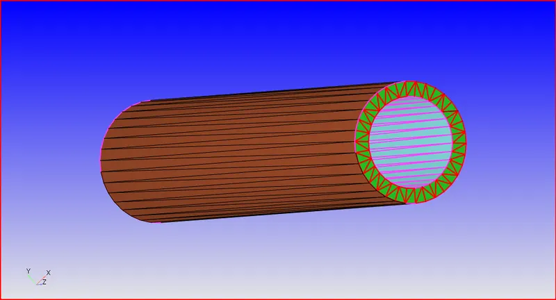
Assign to the boundary.
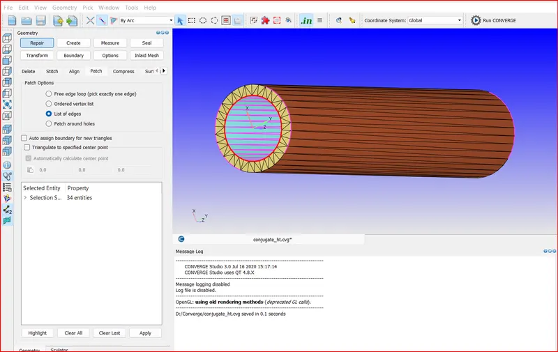
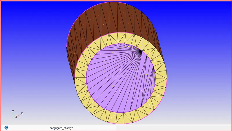
Repair> patch> list of edges> select by arc.
On running the diagnosis check we can see non manifold problems and is normal in cht problems.
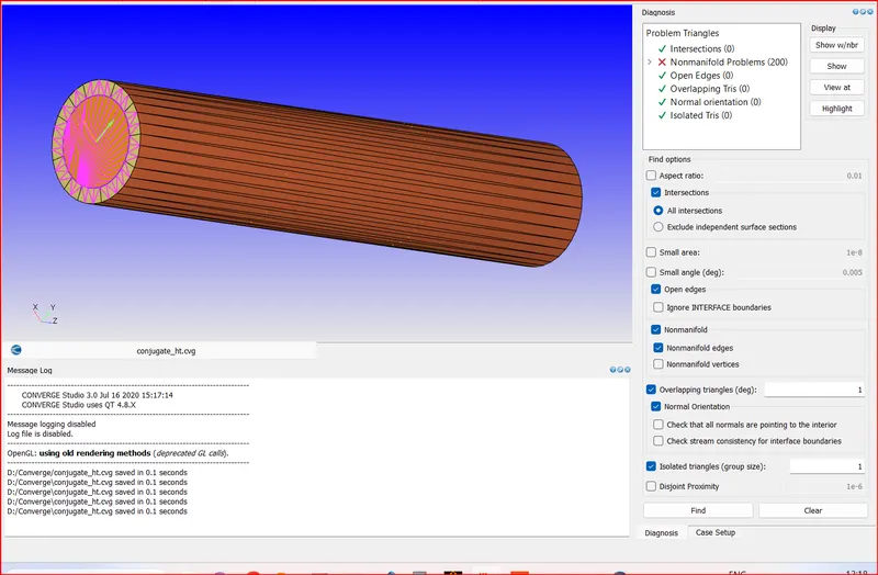
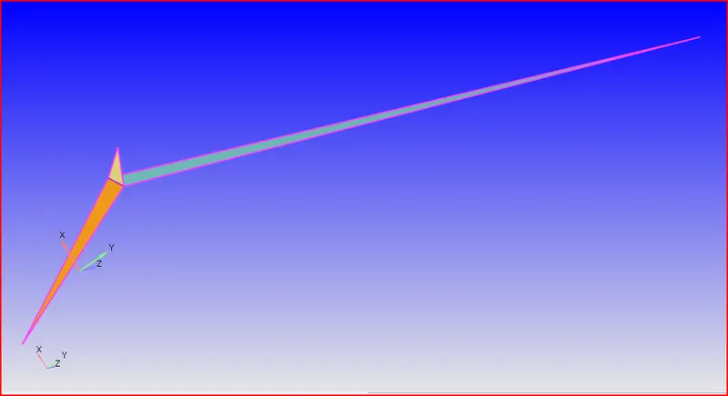
In the above pic we can see that the edge is shared by the three triangles. this is causing the non manifold edges.
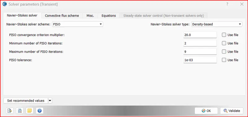
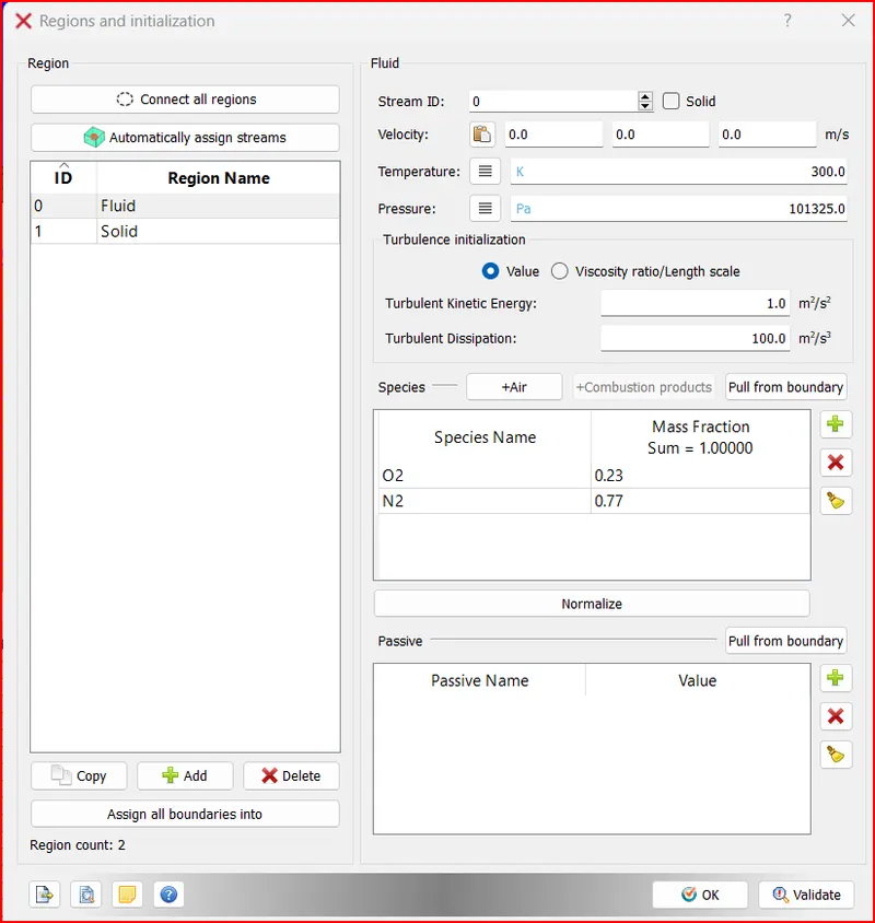
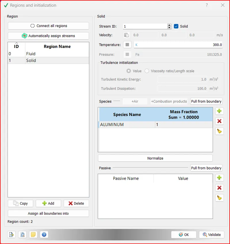
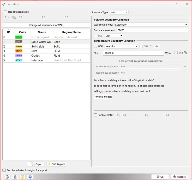
Case Setup:
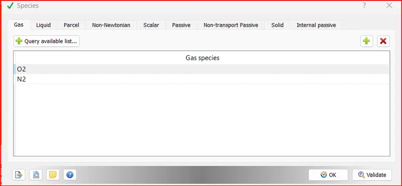
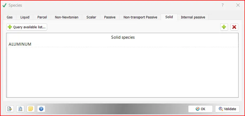
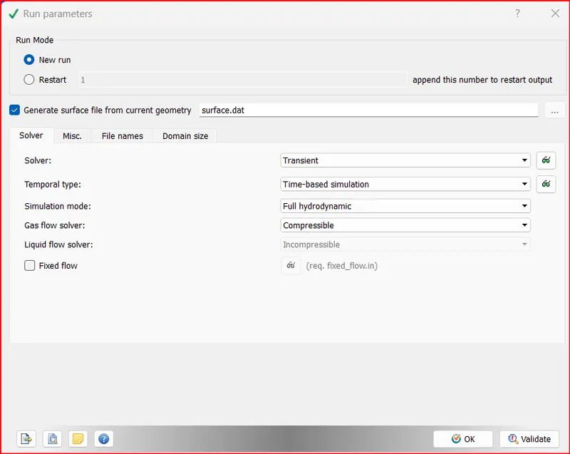
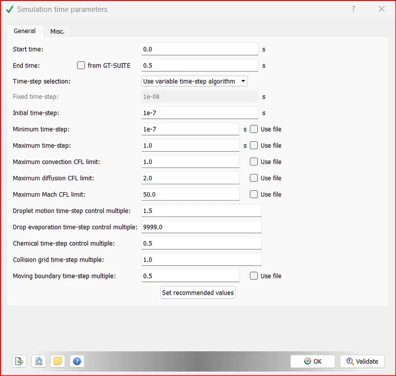
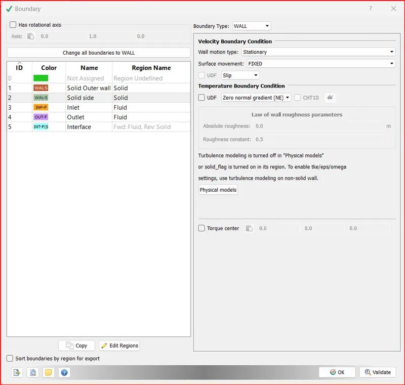
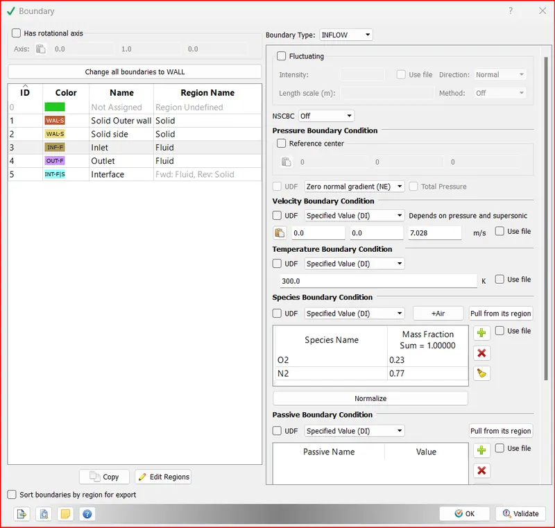
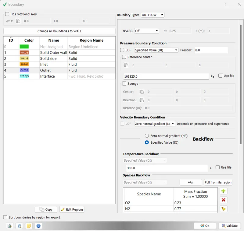
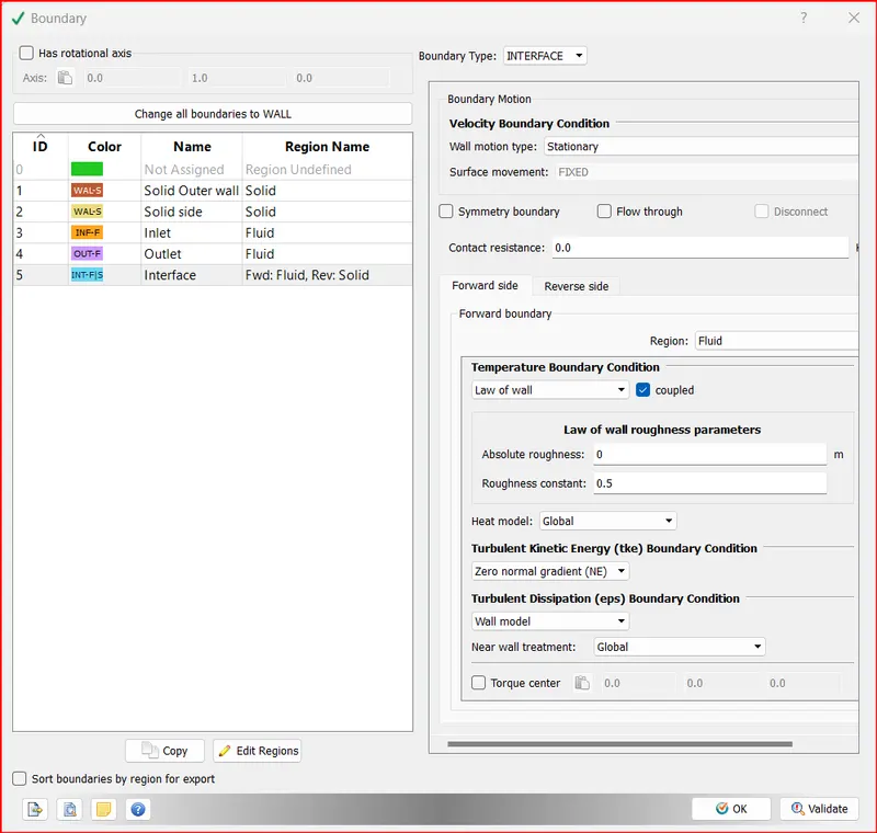
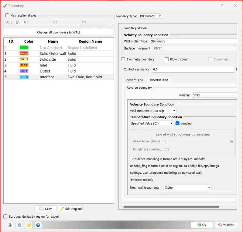
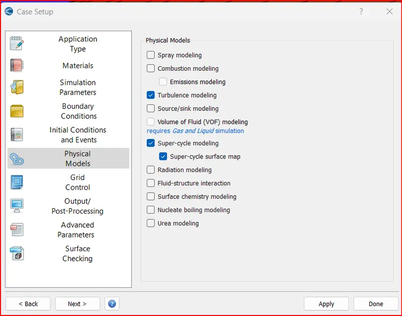
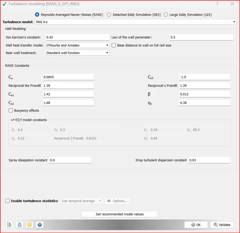
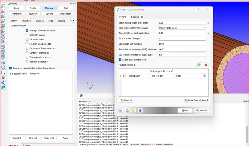
Post Processing:
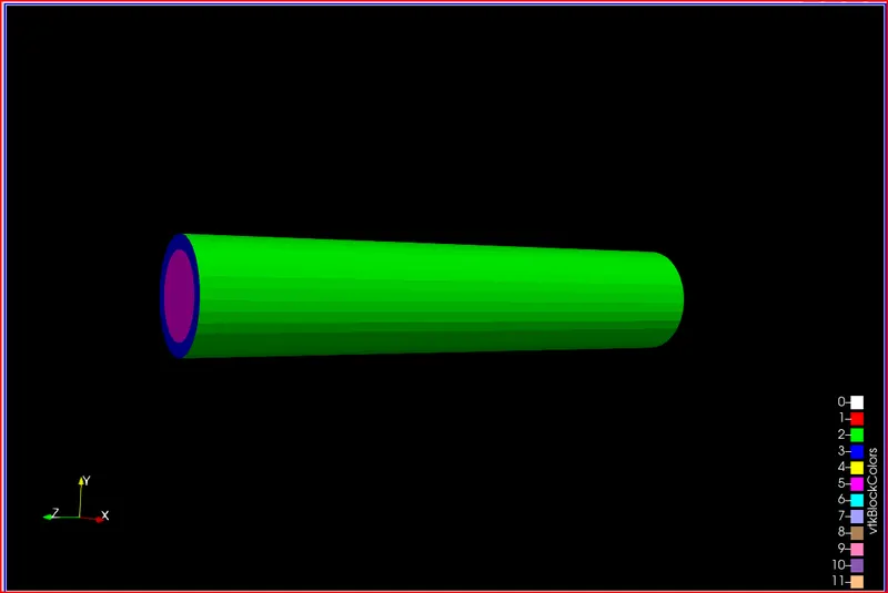
In paraview load .vtm file and click on apply.
in view go to Multi block Inspector and uncheck cell data.
Results:
Case-1 Base mesh
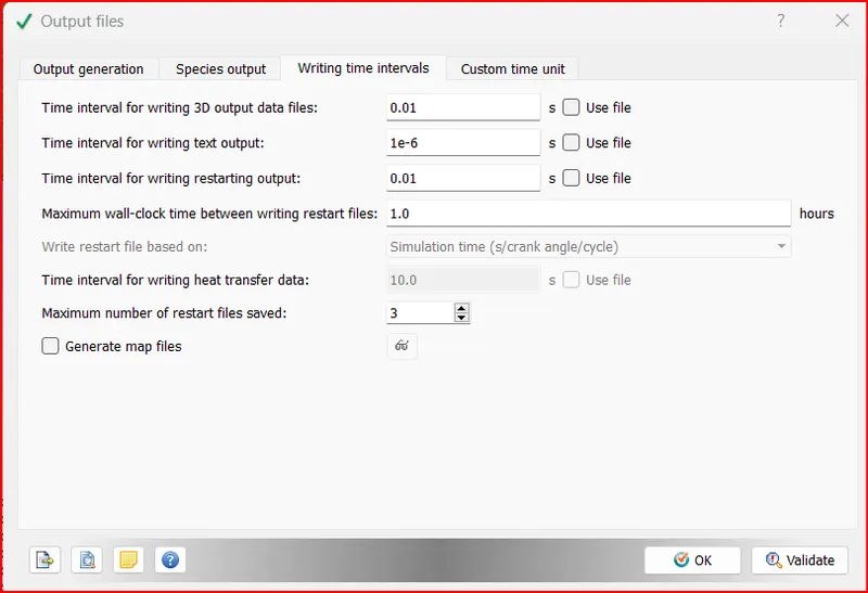
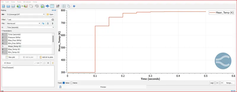
supercyle stage interval 0.01
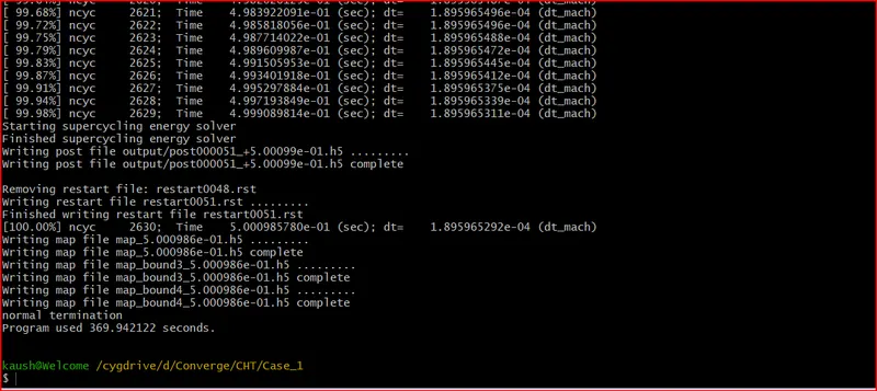
Mean Temperature plot:
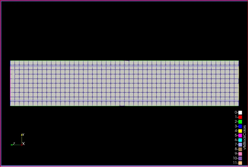
Mesh:
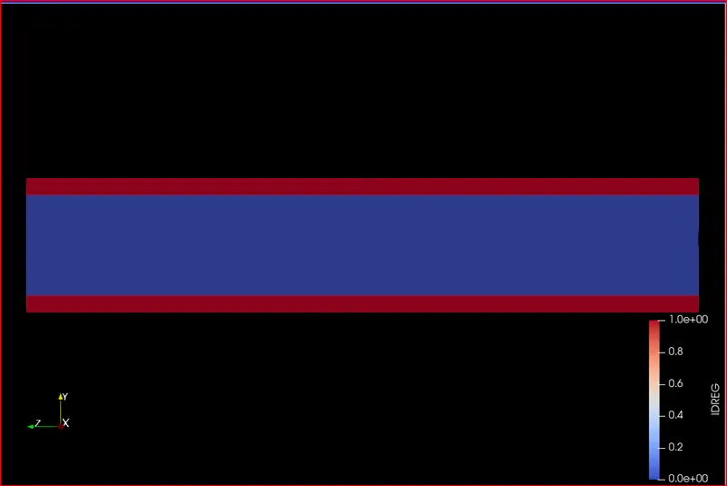
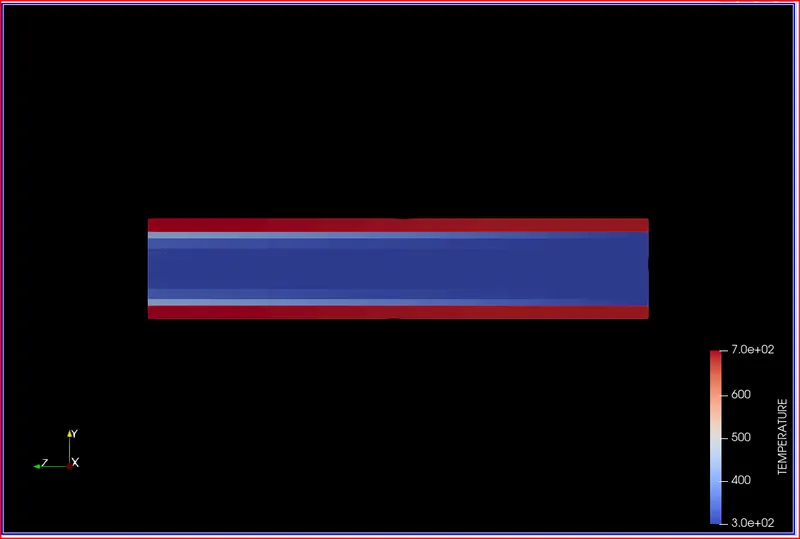
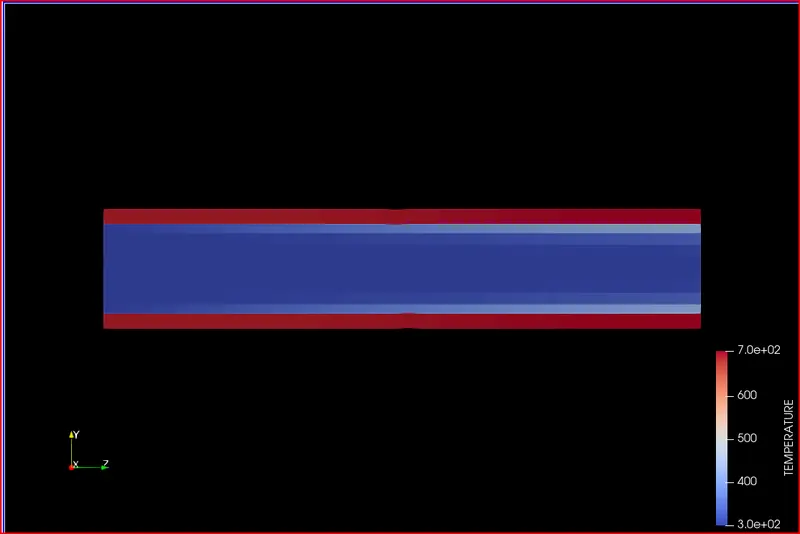
Temperature contour
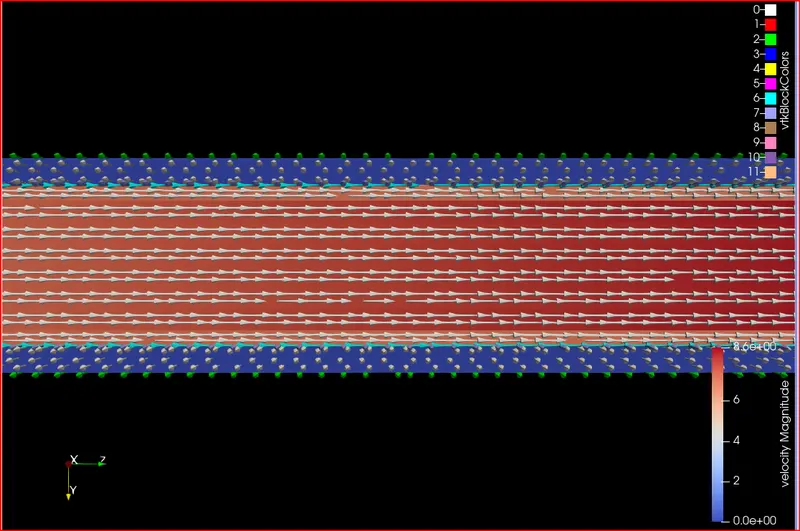
Velocity vector
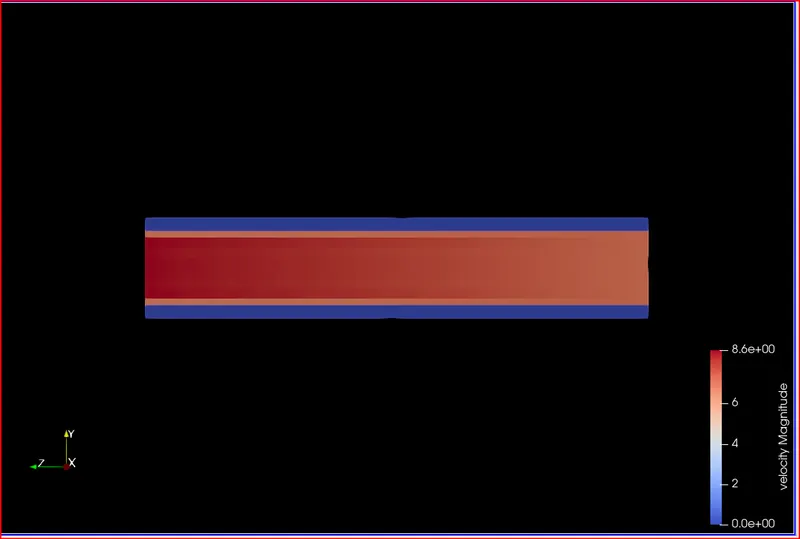
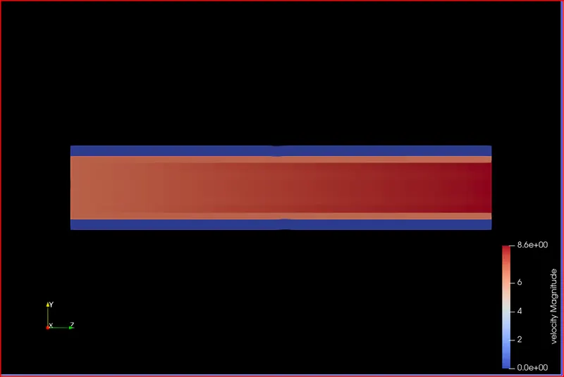
Velocity Contour
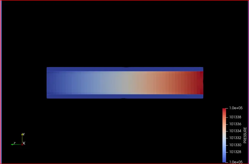
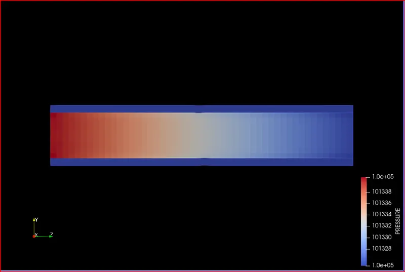
Pressure contour
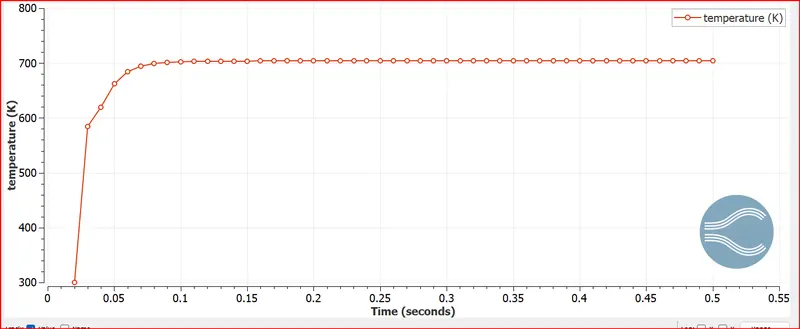
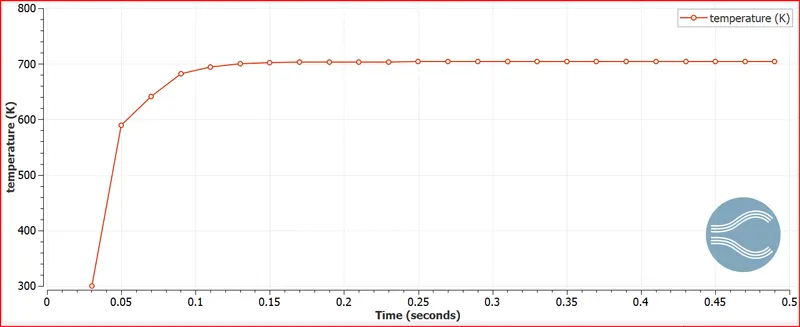
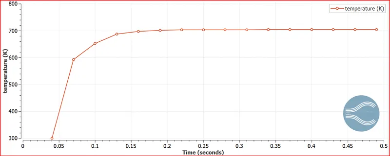
Supercycle monitor point temperature
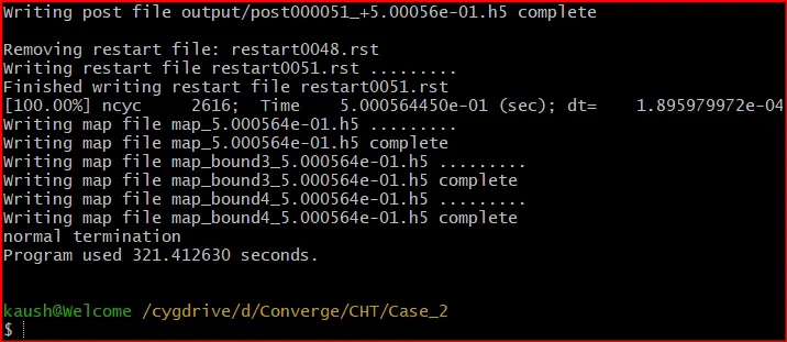
supercyle stage interval 0.02
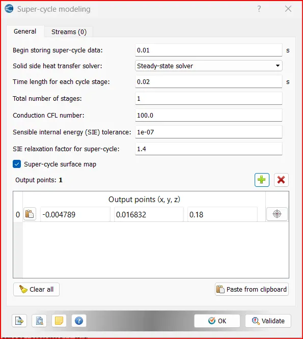
Simulation Run Time
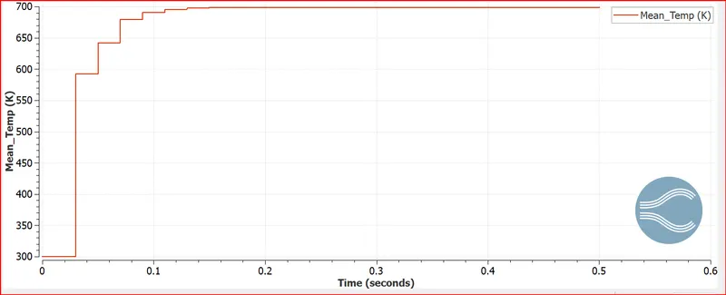
Solid region Mean temp:
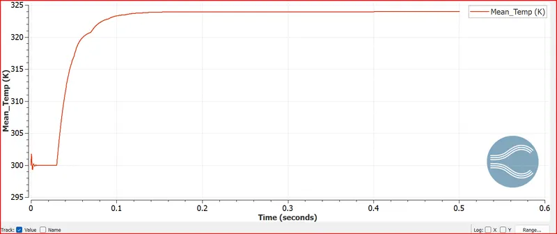
Fluid region Mean temp:
Mesh
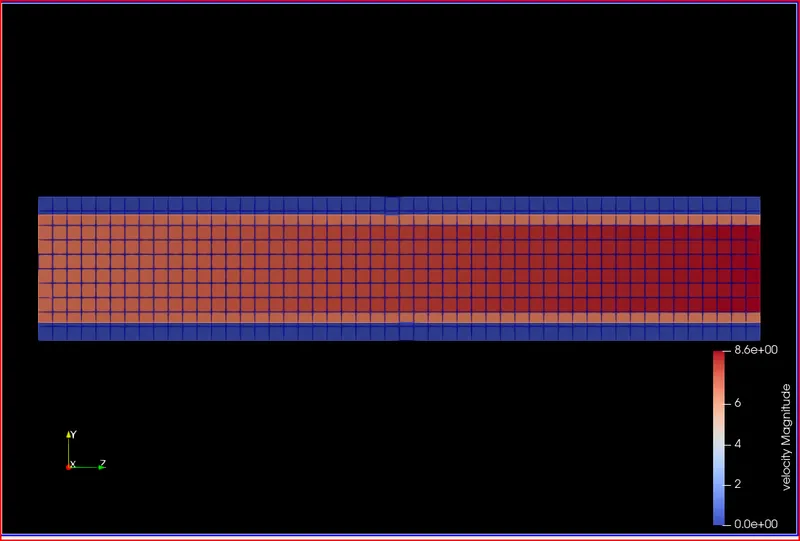
Velocity Contour
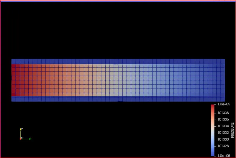
Pressure Contour
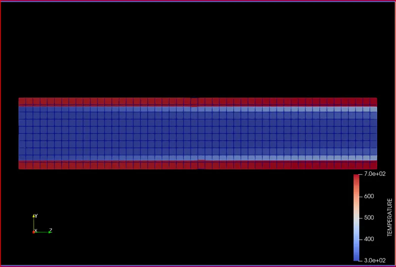
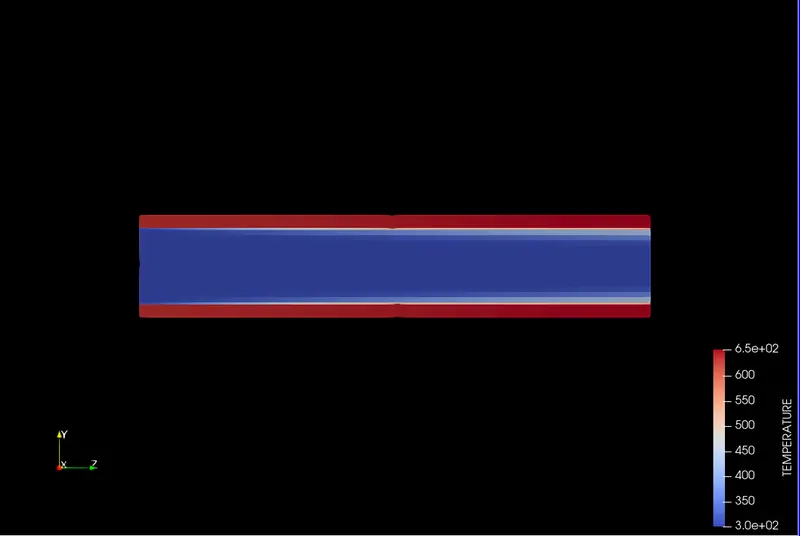
Temperature contour
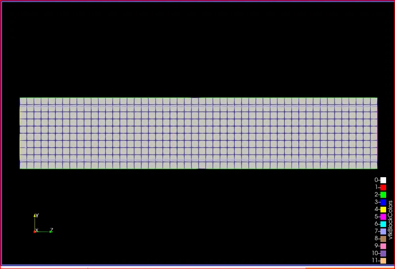
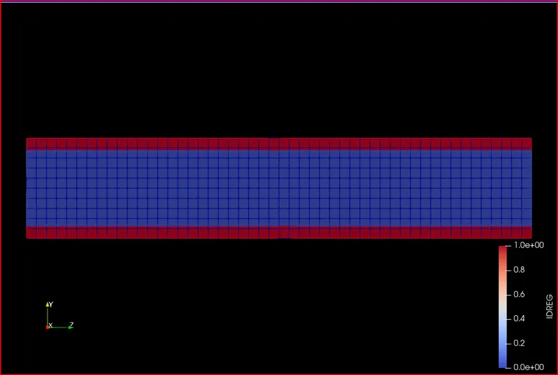
Id Region:
Monitor Point Temperature
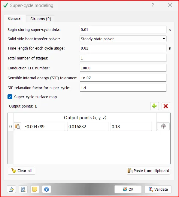
supercyle stage interval 0.03
 .
.
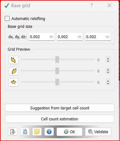
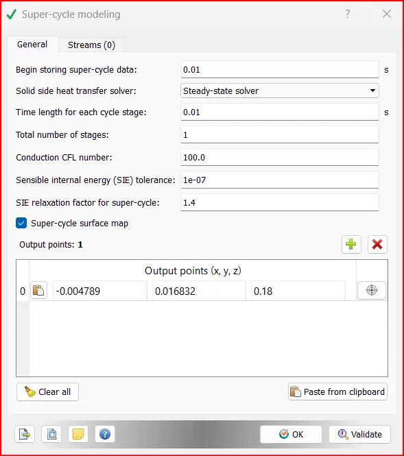
Case 2 Mesh of size 0.002
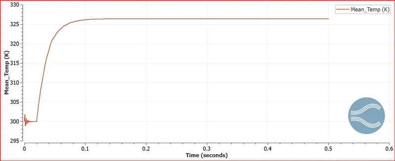
Fluid reg temp:
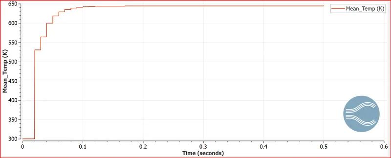
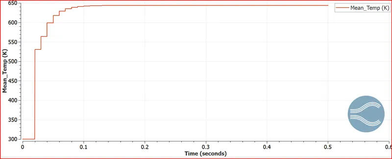
Solid Region temp:
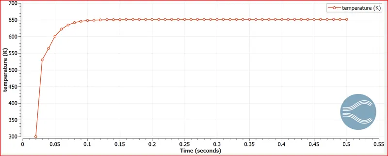
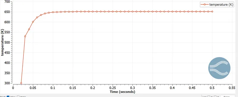
Monitor point temperature:
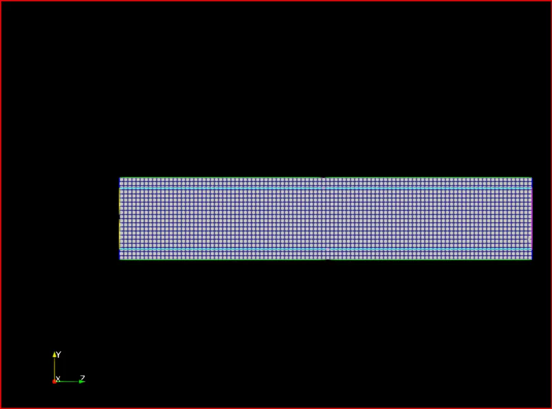
Mesh:
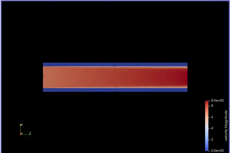
Velocity Contour
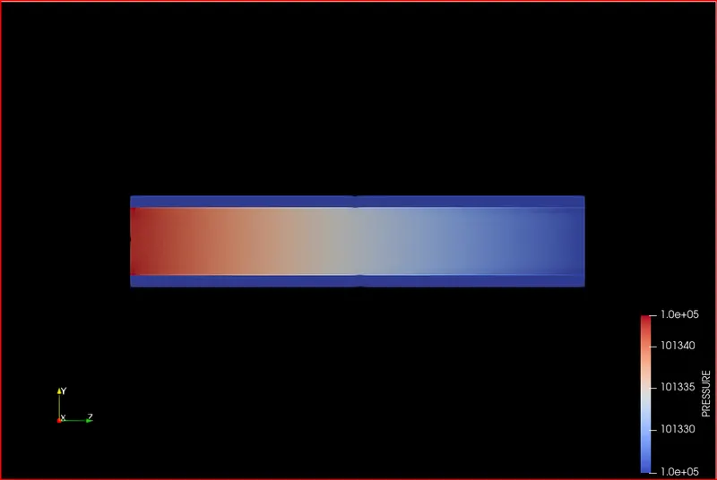
Pressure contour
Temperature contour
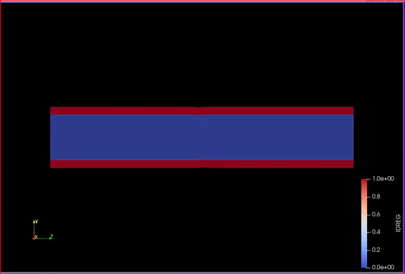
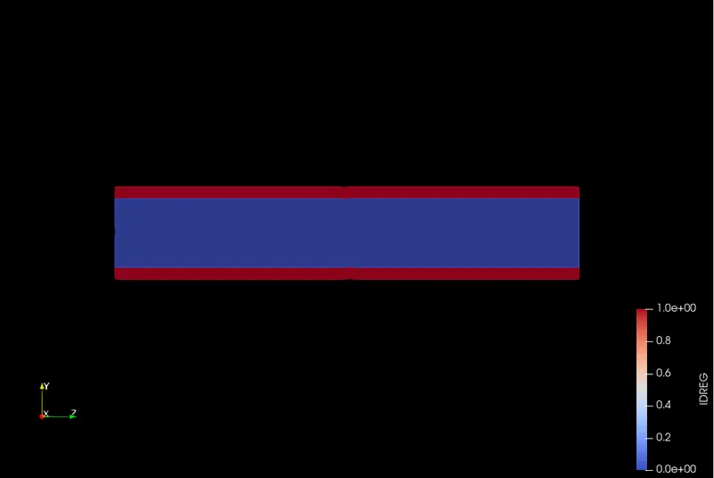
Id regions
Temperature plot solid region:
Monitor point temperature:
Animation https://youtu.be/WZI1_55gv4w
Case 3 Mesh of size 0.001
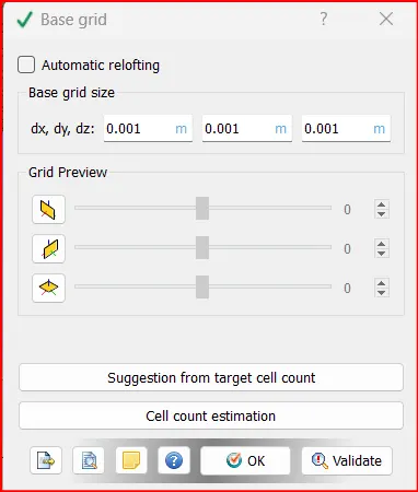
Mesh
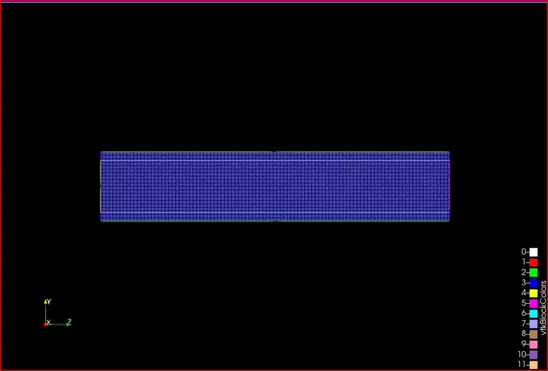
Velocity Contour:
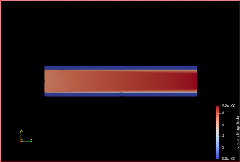
Temperature contour:
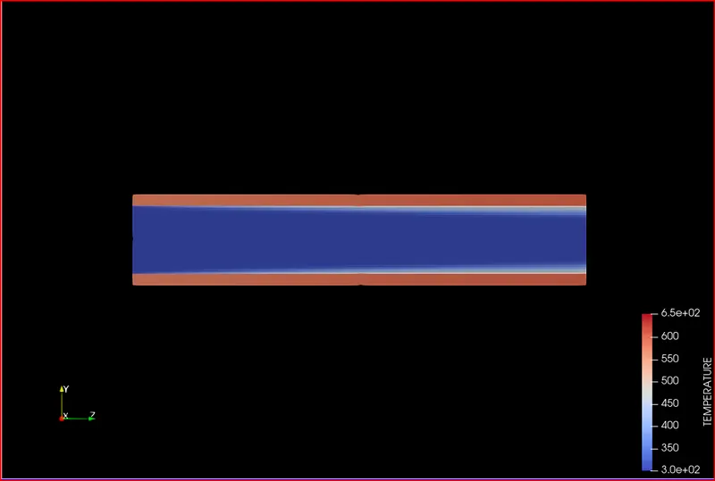
Pressure contour
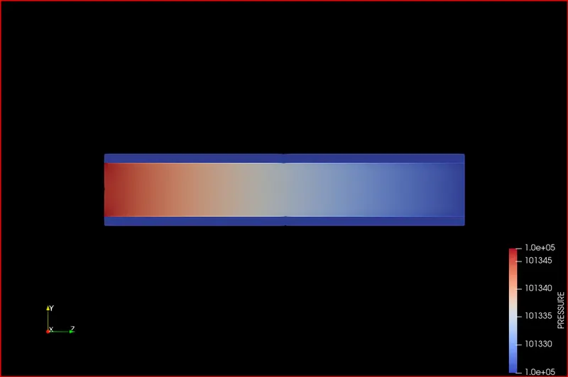
Id region
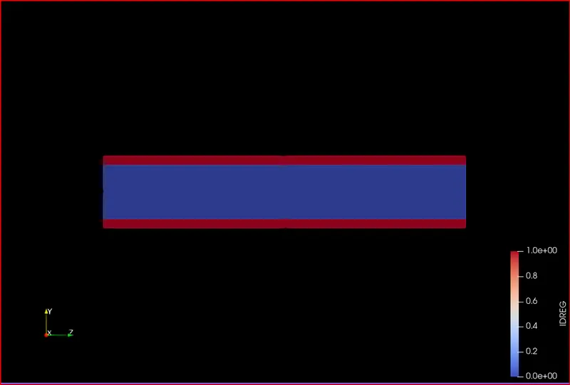
Mean Temp Curve:
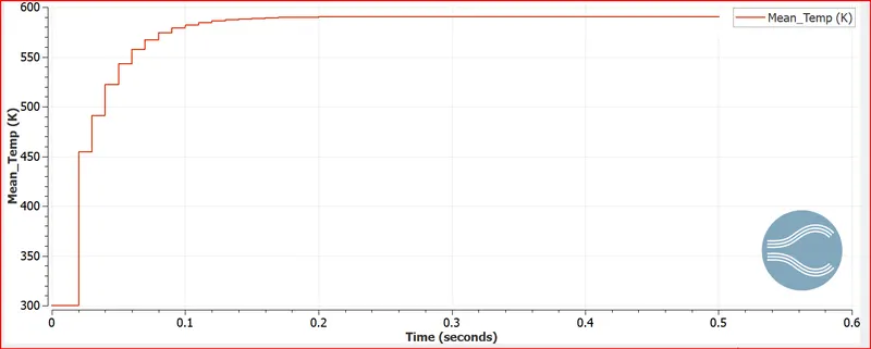
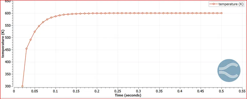
Monitor point temp:
Animation: https://youtu.be/r4dCPF0sujw
Conclusion:
Grid dependency test.
As the mesh length is decreased the monitoring point temperature also decreases.
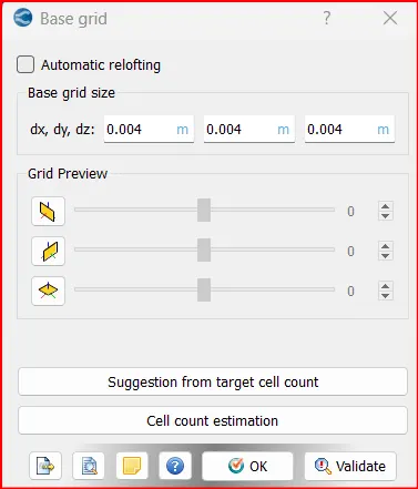
Case 1 mesh size 0.004 mm monitoring point temperature is 700.
Case 2 mesh size 0.002 mm monitoring point temperature is 650.
Case 3 mesh size 0.001 mm monitoring point temperature is 600.