Week 6: Conjugate Heat Transfer Simulation

Aim: To Simulate the flow through the solid pipe “ Conjugate Heat Transfer Simulation “ and understanding the super cycling.

We have to perform a base line configuration

Setup a flow simulation through a pipe

Inlet Reynolds number should be 7000

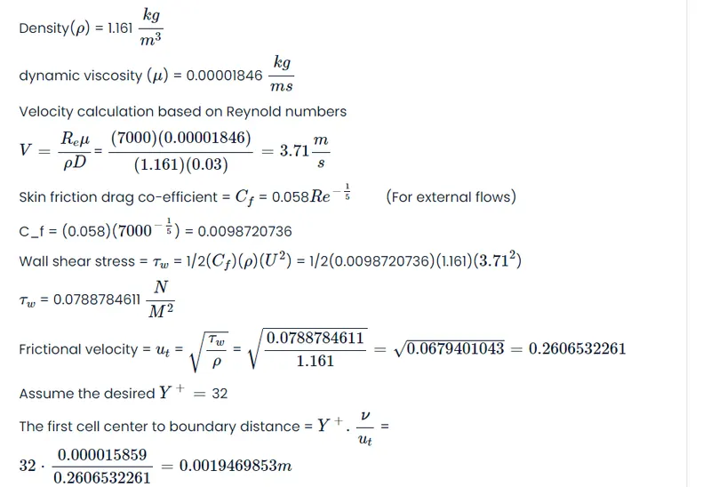
Hint: Use the below formula to calculate velocity for corresponding value of Reynolds Number and give DIRICHLET BC for velocity at inlet and specify the value for velocity calculated at inlet BC using below formula

Re=(rho*V*D)/(Dynamic viscosity)

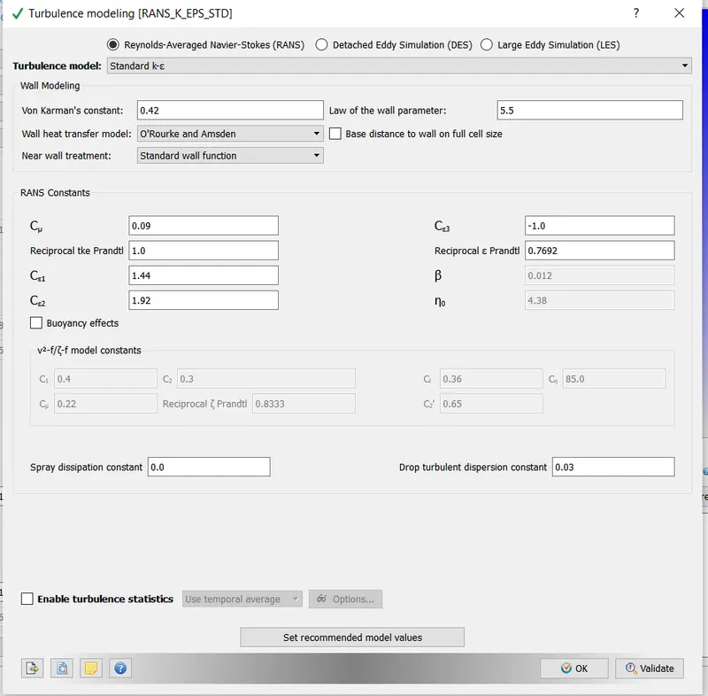
Turbulence modelling -k-Epsilon

Supercycling Parameters-same as its

Additional 3D Outputs

Add Y+to your post.in file

Grid Dependence test

Start with initial base grid

Run grid dependence test on 3 grids and show that the outlet temperature converges to a particular value.

Effect of supercycle stage interval

Set supercycle stage interval of 0.01,0.02,0.03

For these three values , how does the total simulation time compare against the baseline configuration.

Brief of CHT Analysis is used:

The term conjugate heat transfer (CHT) is used to describe process which involve variations of temperature with in solids and fluids , due to thermal interaction between the solid and fluid . The exchange of thermal energy between the two physical bodies is called study of heat transfer, the rate of transferred heat is directly proportional to the temperature difference between the bodies. A typical example is the heating or cooling of a solid body by the flow of air in which it is immersed and some other examples includes conducting through solids , free and forced convection in the gases / fluids and thermal radiations . Typical applications of the analysis of this analysis type exists as but are not limited to the simulations of heat ex-changers , cooling an electronic equipment and general purpose cooling the heating system

Conjugate heat transfer corresponds with the combination of heat transfer in solids and heat transfer in fluids. In solids conduction often dominates and in fluids convection dominates. . Efficiently combining heat transfer in fluids and solids is the key to designing effective coolers ,heaters or heat exchangers rate,In some applications the performances are further improved by combining convection with phase change ( liquid water into vapour phase change)

Heat transfer in solids and heat transfer in fluids are combined in the majority of applications .This is because the fluid flow around solids or between solid walls and because solids are immersed in fluids.

Mode if heat Transfer:

* Conduction:Diffusion of heat transfer due to temp gradients . A measure of the amount of conduction for a given gradient is the heat conductivity.

* Convection:When heat is carried away by moving fluid. The flow can either be caused by external influences , forced convection or by buoyancy forces , natural convection Convection heat transfer is tightly coupled to the fluid flow solution.

* Radiation:Transfer of energy by electromagnetic waves between the surfaces with different temperature , separated by a medium that is at least partially transparent to the infrared radiation Radiation is especially important at high temperature e.g during combustion process but also have a measurable effect at room temperature.

An accurate description of heat transfer modes,material properties flow regimes and geometrical configuration enables the analysis of temperature fields and heat transfer.

Typical design problem involve the determination of: Overall heat transfer efficient , e.g for a car radiator

* Highest or lowest temperature in a system , e.g gas turbine, chemical reaction, vessels

* Temperature Distribution (related to the stress) e.g in the walls of a space craft.

* Temperature response in the time dependent heating/cooling problems e.g Engine cooling, or how fast does the car heat up in the sun and how is it effected by the shape of the windshield.

The fluid flow and heat transfer problems can be tightly coupled through the convection term in the energy equation and when the physical properties are temp dependent while analytical solutions exist for some simple problems , we must rely on computational methods to solve most industrially relevant applications.

CHT can be performed to improve cooling performance of the water jacket and increase the engine life. Advance in cooling for applications such as gas turbines components required to improve understanding of the complex heat transfer mechanism and the interactions between those mechanism , which our engineers can perform without hassle. Critical cooling often relay on multiple thermal protection techniques including internal cooling external film cooling etc.,, Which are efficiently used by our analysis to cool components and limits in the use of coolant . we do extensive support for motor and battery CHT analysis to get optimized design for high voltage systems. CHT analysis provides the temp distribution in the solid, coolant of the engine, and clear insight of velocity distribution and mechanism of heat transfer of coolant. Result of CHT analysis become input to structural simulations as thermal loads.

We have a wide experience in Engine CHT Analysis of various types of engine like bikes, Passenger cars ,Racing cars, Commercial vehicles ,marine..,

Mathematical Modelling:

The flow of thermal energy from matter occupying one region in space to matter occupying a different region in space as heat transfer . The heat transfer can occur in three methods.

* Conduction

* Convection

* Radiation

Physical models involving conduction / convection only are the simplest while buoyancy - driven flow or natural convection and radiation models are complex.

Super Cycling Concept:

Super cycling is a technique which is used in converge studio in the case of CHT problems with a solid and liquid regions. Main problems in that both solvers cannot run at the same speed since solving in fluid domain in such a much faster owing to time scale. Difference for heat transfer in liquids as compared to solids side . This cause problems during the solutions given that the solid side solver would not have reached a steady state converge in the time the liquid solver does. This is where the concept of super cycling is based.

The basic idea of super cycling is that the solver for the fluid domain is paused until the solver for the solid domain converges

These steps are to be follows:

* Solve the fluid and the solid together with the transient solver, Store the instantaneous heat transfer coefficient and temperature on the interface during process.

* freeze the solver Time-average the heat transfer coefficients and temperature and applies them as boundary conditions at the interface.

* Solves the solid temperature until it reaches steady-state.

* Update the solid temp field and unfreeze the fluid solver.

* Repeat until the solid temp converges.

Calculate velocity at the inlet based on Reynolds Number:

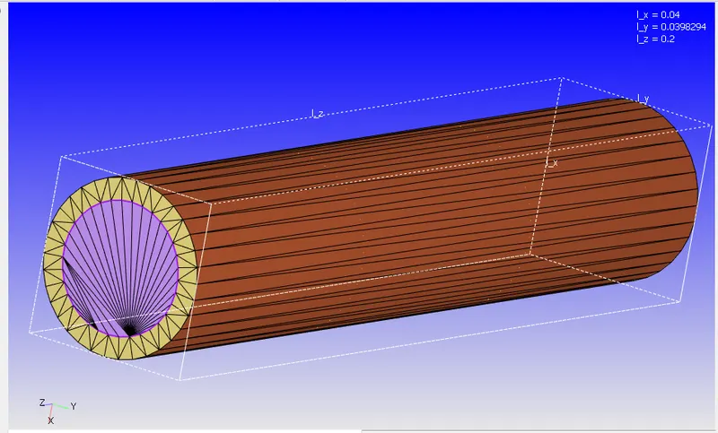
Geometry Dimension:

Internal Dia:0.03 m

Thickness:0.01 m

Length Of the Tube:0.2m

Geometry Setup:

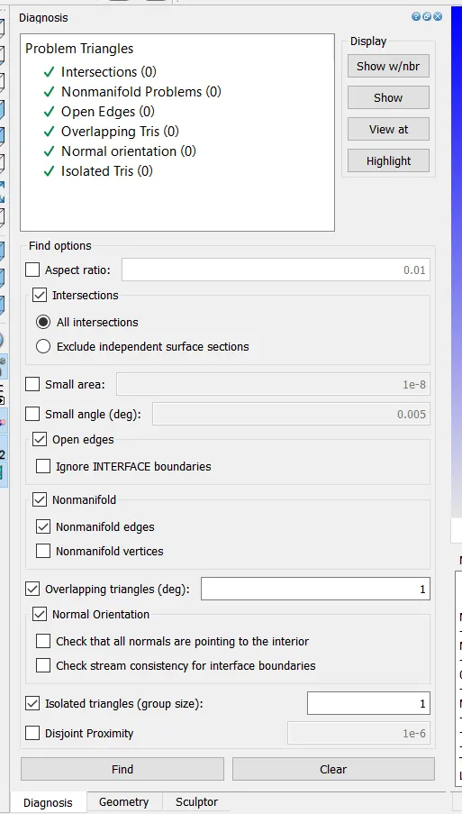
Check for Diagonasis:

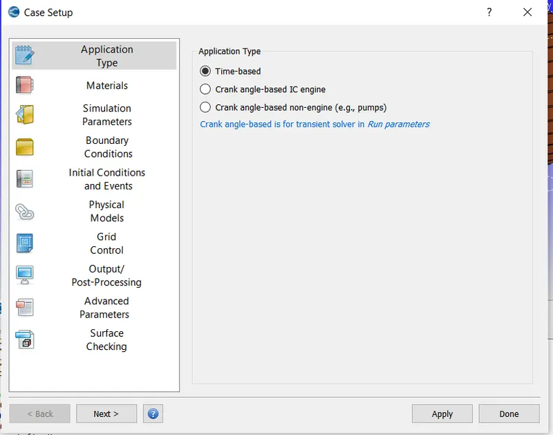
Case Setup:

Material selection:

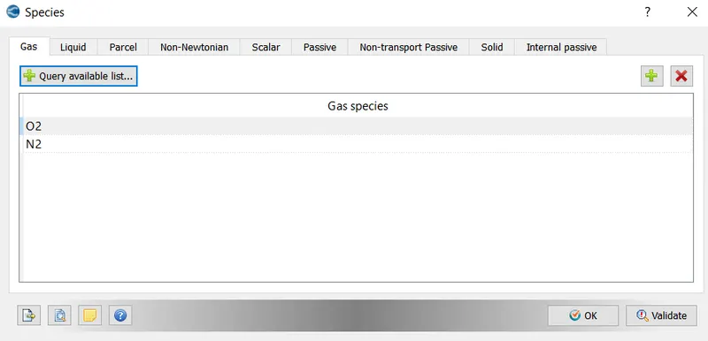
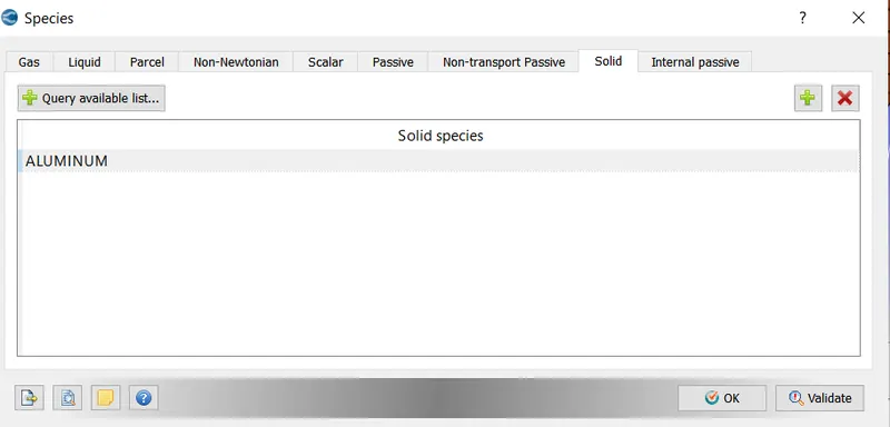
In this setup Gas and solid silumtion are selected to define the CHT analysis.

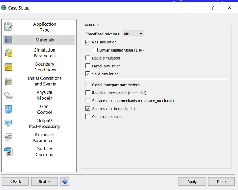
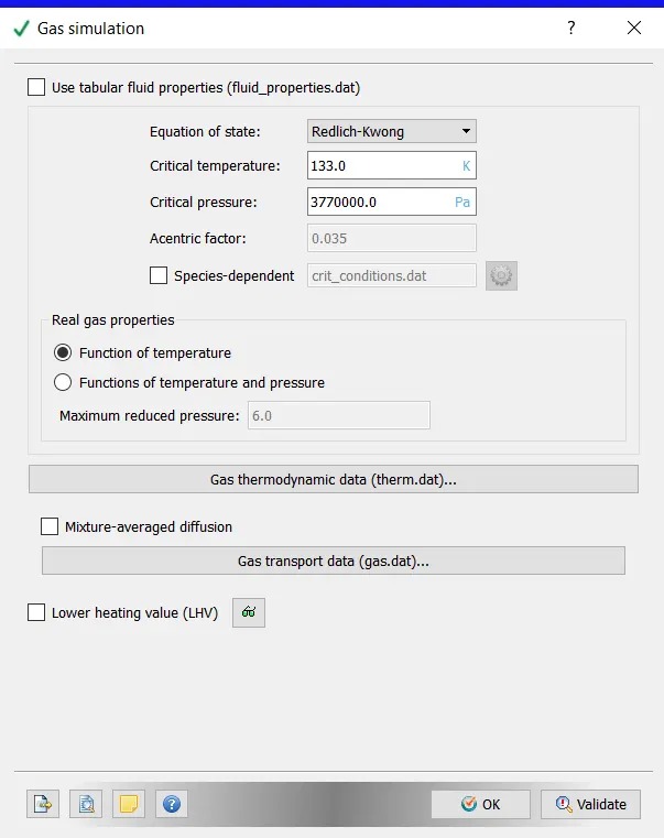
Gas Simulation:

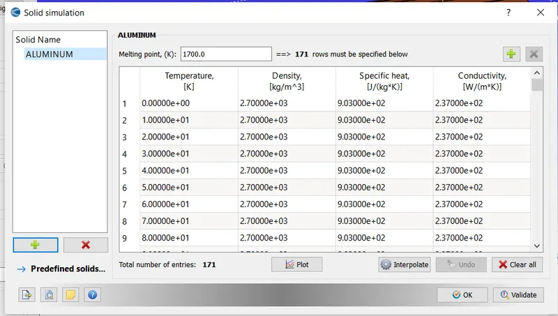
Solid Simulation:

Where we can see the material Properties of the Aluminimum for the solid state

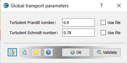
Global Transport Properties:

The Proeprties are set as default and no changes

Species:

Gas :

Solid:

Simulation Parameters:

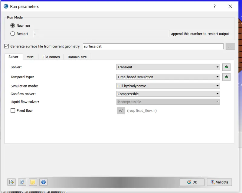
Run Parameters:

The model set as transient Mode

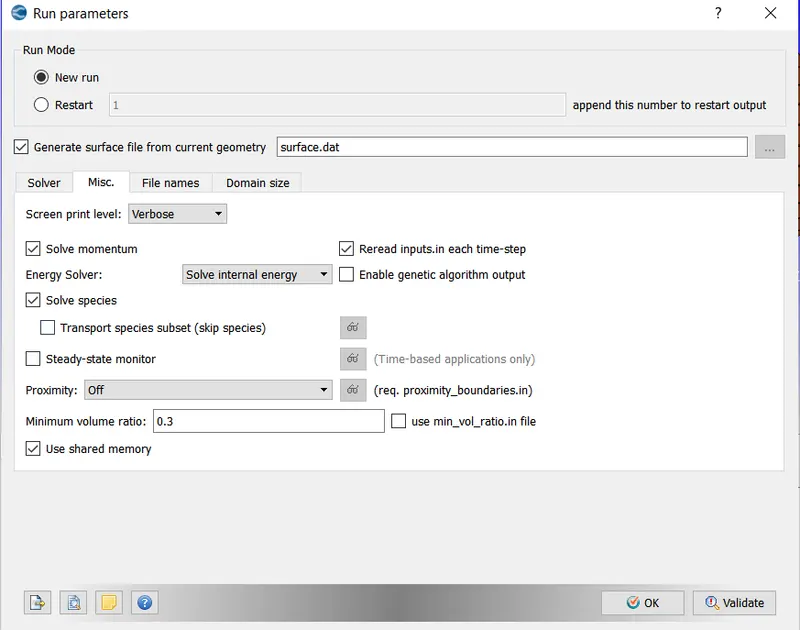
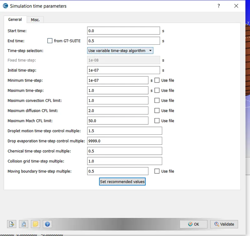
Simulation Time parameters:

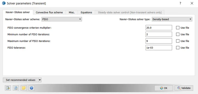
Solver Parameters:

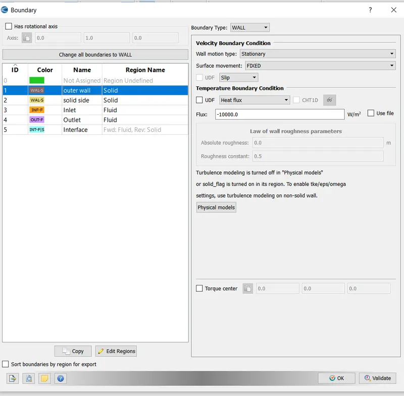
Boundary:

Outer wall:

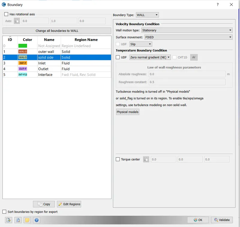
Solid side wall:

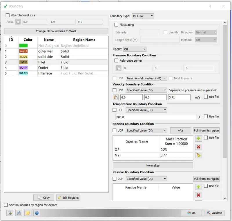
Inlet:

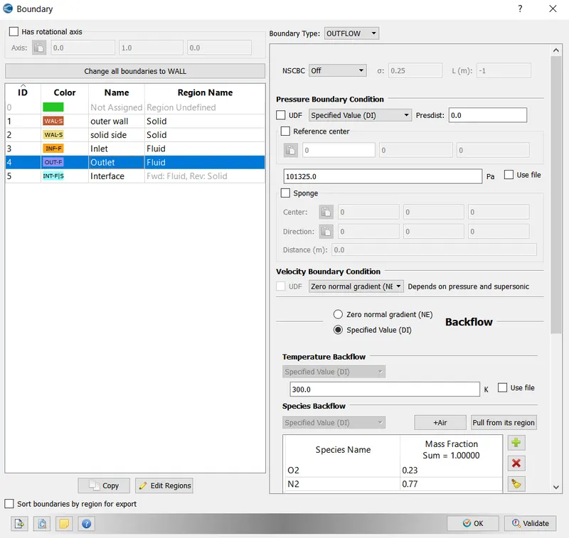
Outlet:

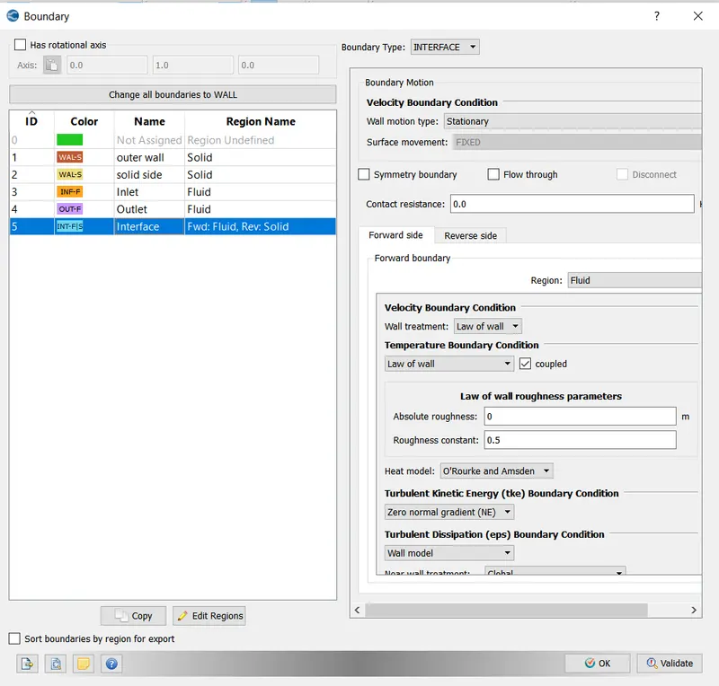
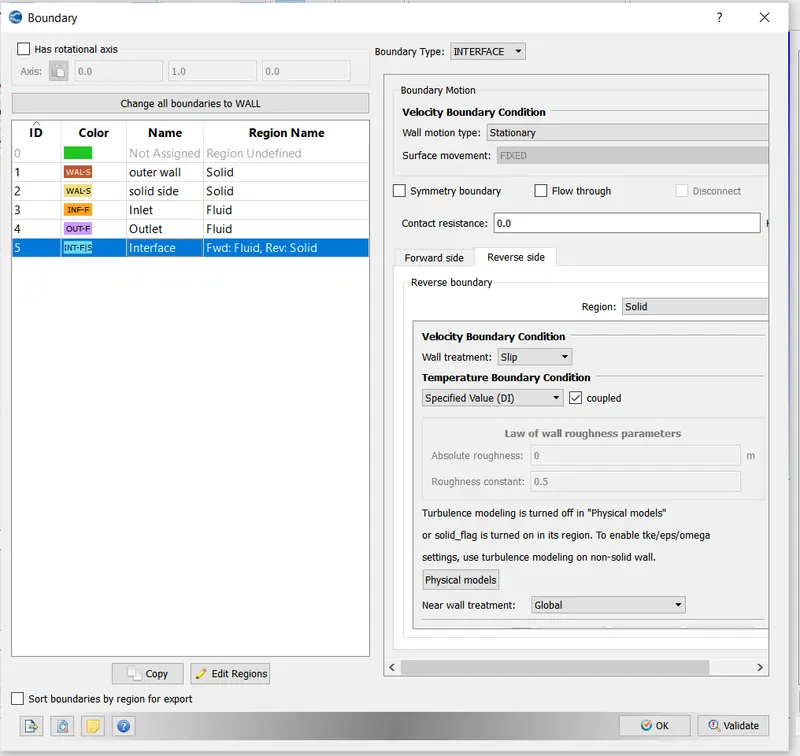
Interface:

Forward:

Reverse:

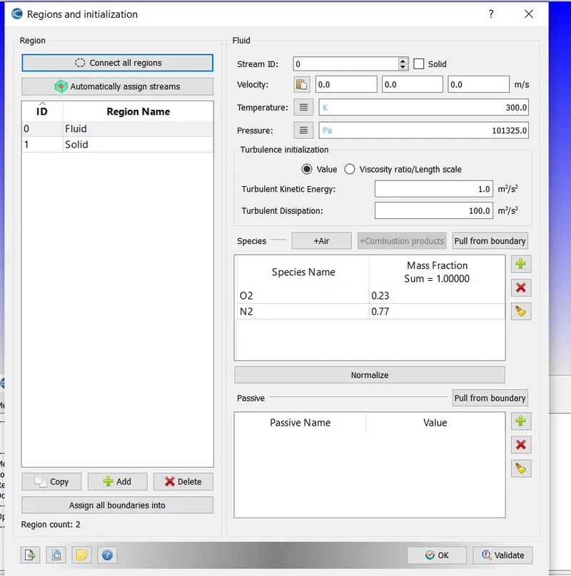
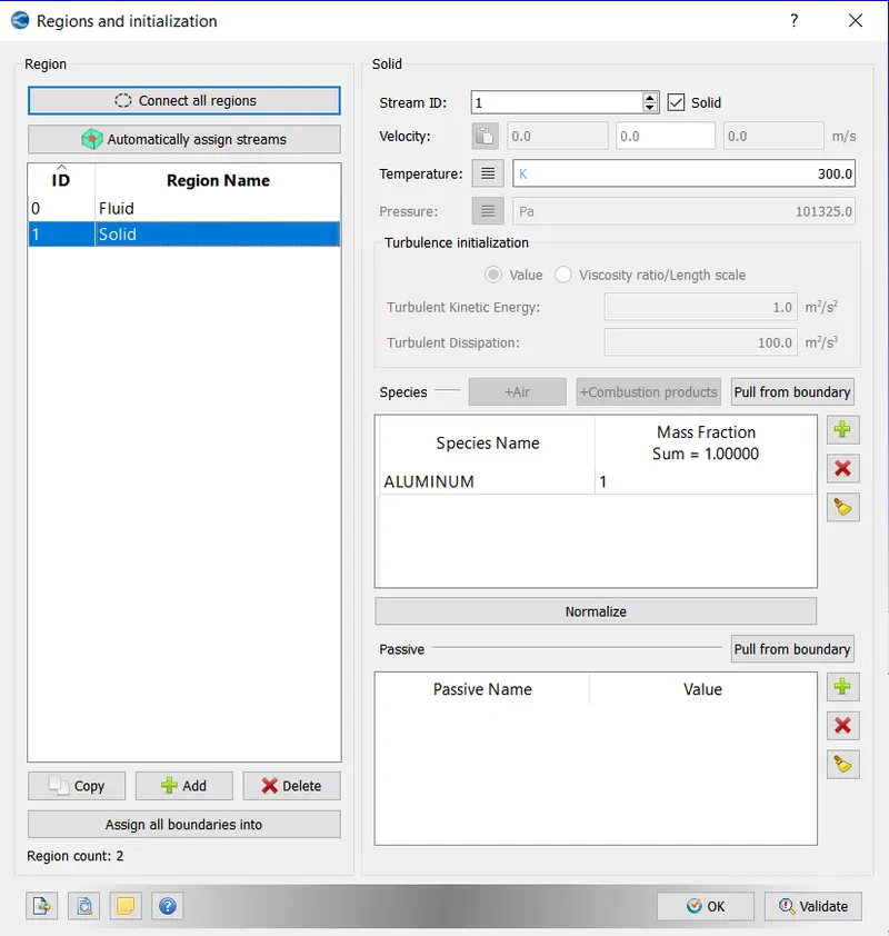
Region and Initilization:

Fluid:

Solid:

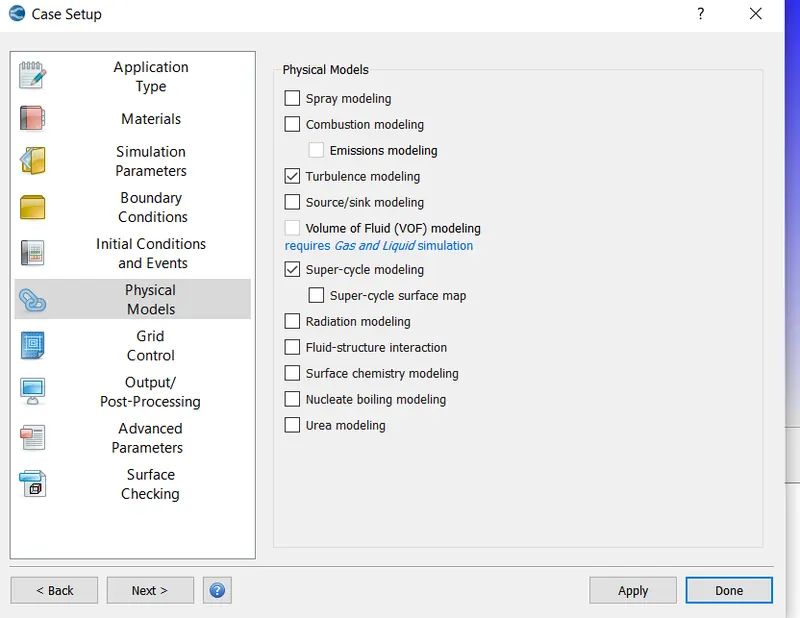
Physical model:

Turbulence Modelling:

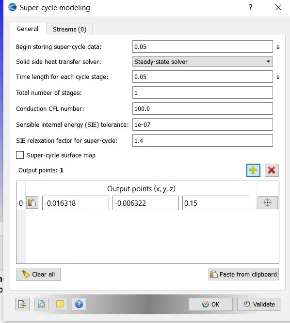
Super cycling:

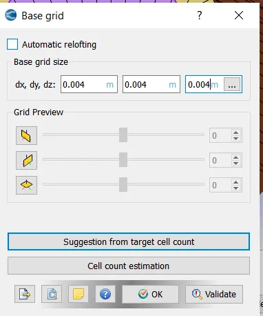
Base Grid:

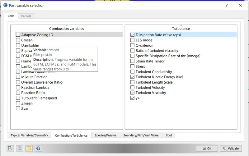
Post Variable selection:

In post Variable selection Y+ also selected to converge

Output files:

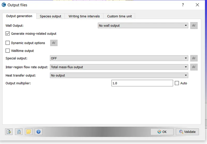
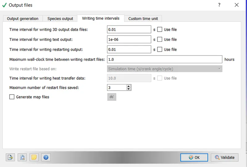
Post case setup the files are exporeted and converge by using CYGWIN to obtain the result of the input

And after the Cygwin Result , By using Paraview the results images are obtained.

Result:

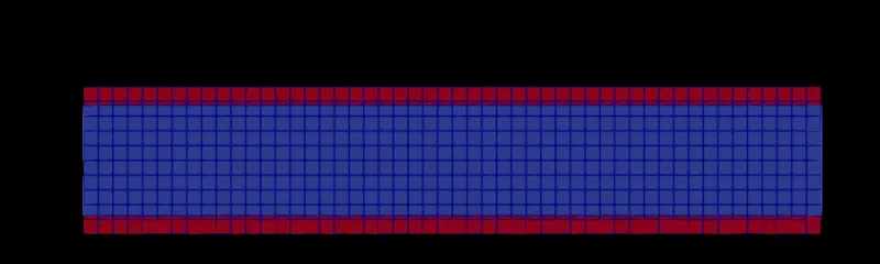
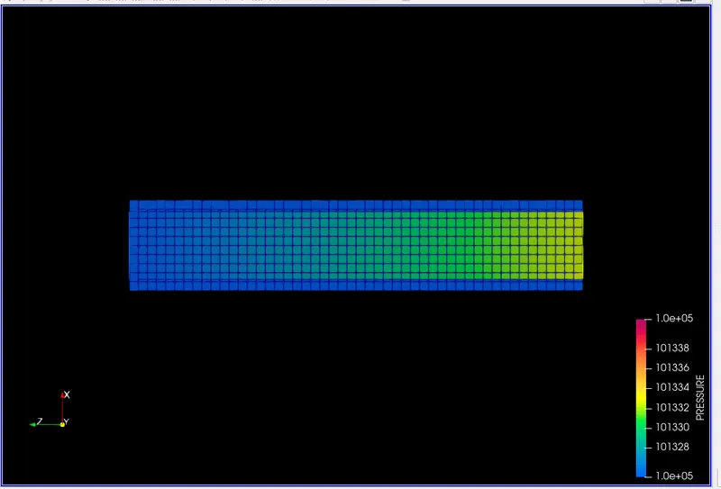
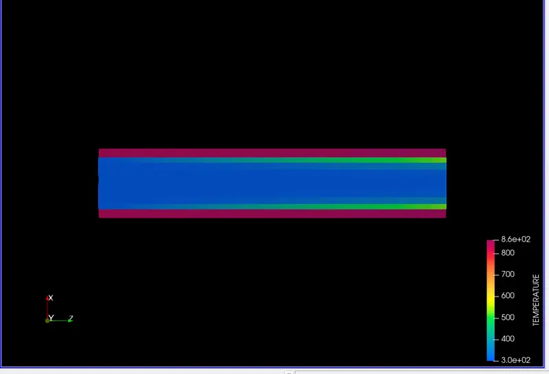
1.) Base set of dx=dy=dz=0.004 m

Mesh:

pressure contour:

Temperature contour:

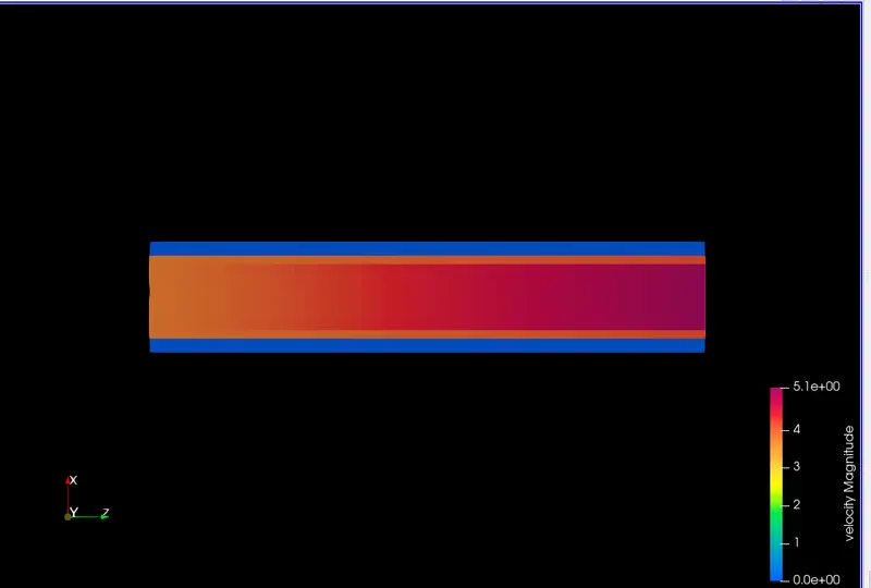
Velocity contour:

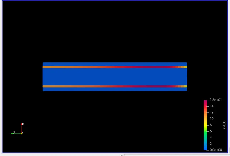
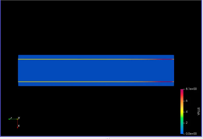
y+ Contour:

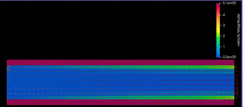
Velocity vector:

2.) Base set of dx=dy=dz=0.003 m

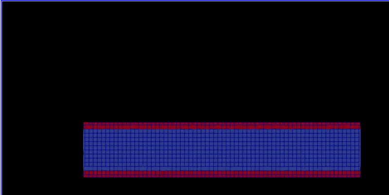
Mesh:

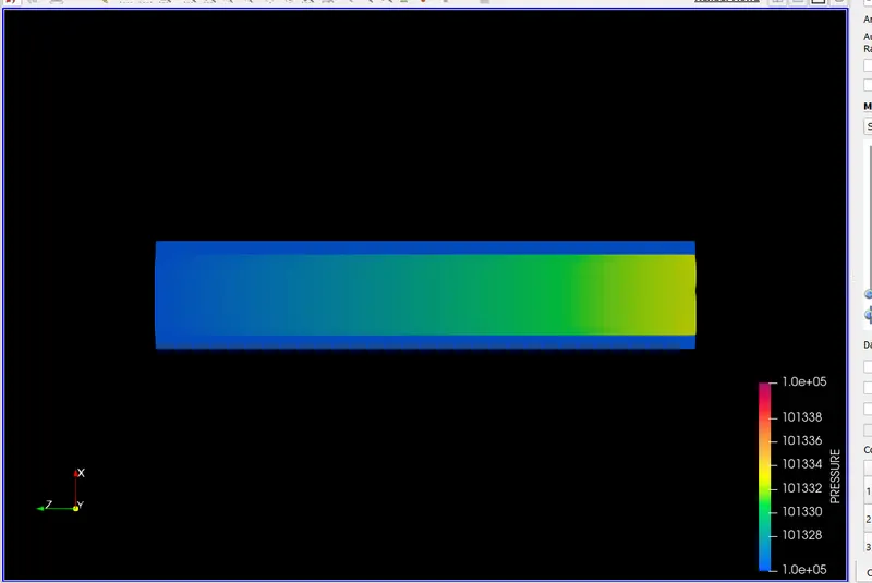
pressure contour:

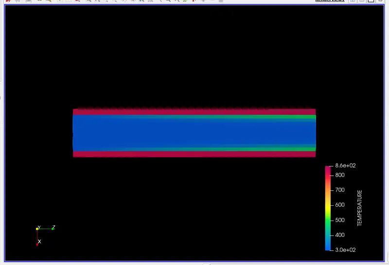
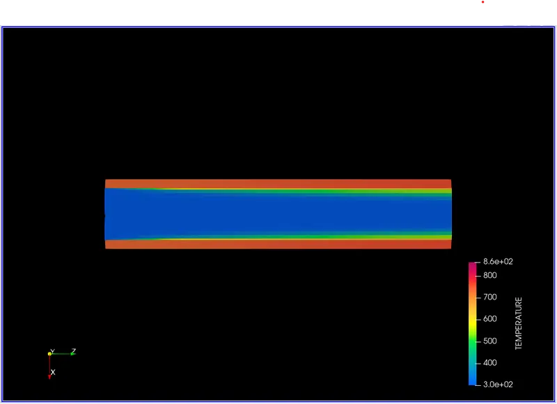
Temperature contour:

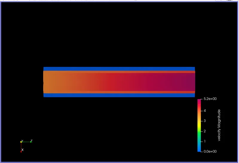
Velocity contour:

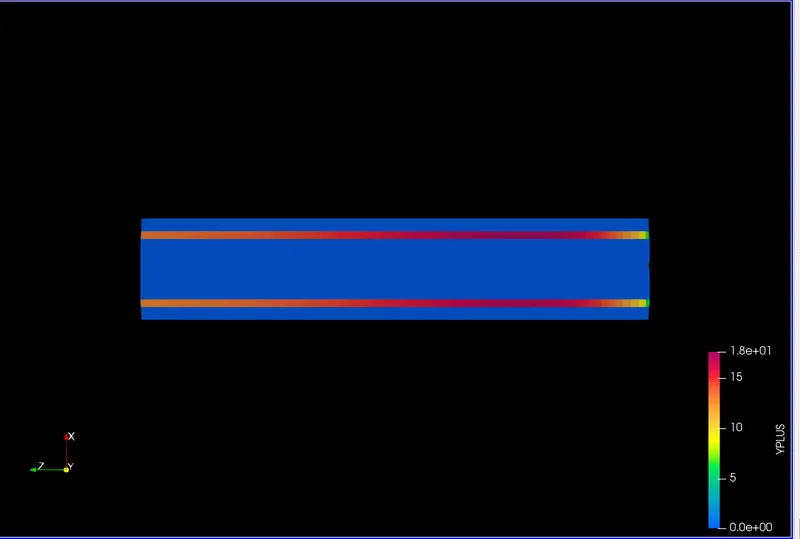
y+ Contour:

3.) Base set of dx=dy=dz=0.002 m

Mesh:

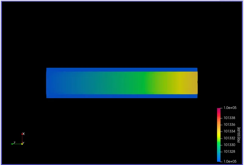
pressure contour:

Temperature contour:

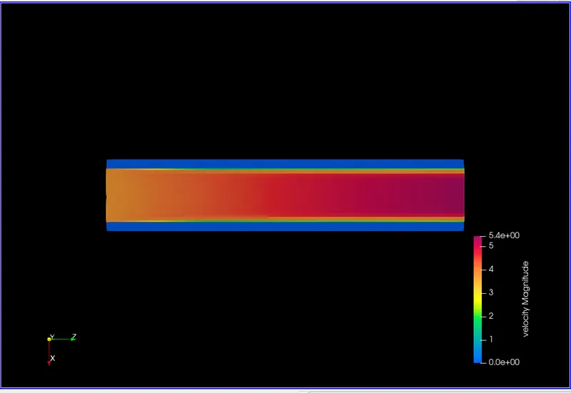
Velocity contour:

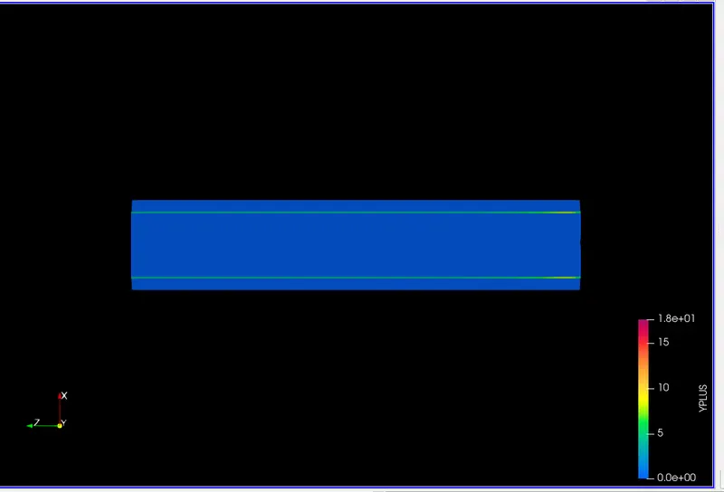
y+ Contour:

4.) Base set of dx=dy=dz=0.001 m

Mesh:

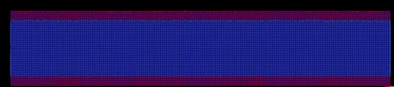
pressure contour:

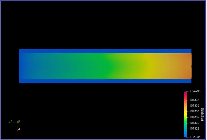
Temperature contour:

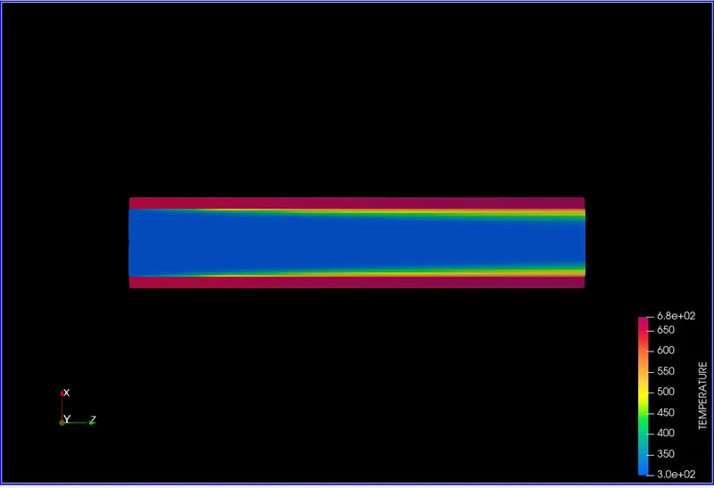
Velocity contour:

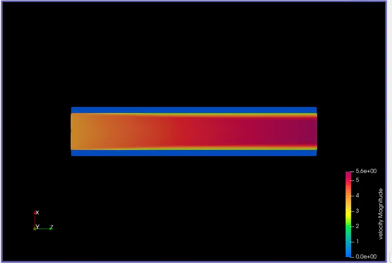
y+ Contour:

Animation:

Pressure Contour

case1:0.004 m

https://drive.google.com/file/d/1PAoGePJMFH3FEyiwr-GwjN-r5vjp_KYj/view?usp=sharing

case2:0.003 m

https://drive.google.com/file/d/1YAi66T37wiK4S_zgh6DlPCx0exJGLr-6/view?usp=sharing

case3:0.002m

https://drive.google.com/file/d/1p_jD46-NtoNcaNzCDIamUDOTx2t6gD5H/view?usp=sharing

case4:0.001m

https://drive.google.com/file/d/1YdYlIIneGg_LDK7jUwfSBu9eAAp9v3cQ/view?usp=sharing

Temperature Contour:

case1:0.004 m

https://drive.google.com/file/d/1LeNPehHKBahthZcCSm64RBxPRI2sLDux/view?usp=sharing

case2:0.003 m

https://drive.google.com/file/d/1vM6DPOztz-r-UzrwtAs8c_2F7aHxeG7M/view?usp=sharing

case3:0.002m

https://drive.google.com/file/d/1SE51WQZrYY8JCb78AFmJLKnGC-GfODHn/view?usp=sharing

case4:0.001m

https://drive.google.com/file/d/1SsPPmVt70JZ4YCOP0QJTebZpn-VrToN9/view?usp=sharing

velocity Contour:

case1:0.004 m

https://drive.google.com/file/d/1Cs1FrW9oREHMNP0mkEW8A15Nvh9MC6KX/view?usp=sharing

case2:0.003m

https://drive.google.com/file/d/1fFQFKqU7JwwTzdraNKFBIUQUNsUpyJQ-/view?usp=sharing

case3:0.002m

https://drive.google.com/file/d/1RNMKziHctTtF5rIsOuE9iqYFh0unAIsf/view?usp=sharing

case4:0.001m

https://drive.google.com/file/d/1VnLaX7HWL3HZTZQbRM1SJVtvQxrBLuzP/view?usp=sharing

Y+ contour:

case1:0.004 m

https://drive.google.com/file/d/100Yv_qAELks62n2UOcJmOv5-JAZcp-J9/view?usp=sharing

case2:0.003m

https://drive.google.com/file/d/1lnqYgeWlCfAGCmA-ZEJRugakmKmG6nT3/view?usp=sharing

case3:0.002m

https://drive.google.com/file/d/14MMZQ9n4HPYikJLX0OBL-6AWos1jlt2-/view?usp=sharing

case4:0.001m

https://drive.google.com/file/d/1JOpRHT1T4z2oghOOvfEcdM7ahmw9hO-u/view?usp=sharing

Mesh:

From the above plots we can see that the mesh is getting refined more and more by the lower value and the output of the mesh are seen in above picture.

Y+:

Near wall modelling it is well seen that the Mesh size is small enough because near wall region have large gradients in the solution variables. The wall y+ is a non-dimensional distance similar to local Reynolds number. When solving the CFD simulation , we need to provide the boundary conditions .And for your turbulence equations perform correctly , we need to make sure that for the first cell height in the right location, Inside the boundary layer the Y+is highly useful, Here are few examples, if you take K-epsilon equation that is called high Reynolds number equation . It is not applicable in the scenario, where flow is laminar and flow is laminar inside the viscous sub-layer , And the Y+ is between 1to 10 , K-epsilon model only used in the outer region. Where Y+ is between 30to 100. And Y+ 30 means that you are 30times away from the character length away from the wall.

In the above y+ contours we can easily observe that the flow for the different size of mesh the values the y+ are given in the following table.

Mesh Size	Y+
0.001 m	08
0.002 m	18
0.003 m	18
0.004 m	16

Plot Results:

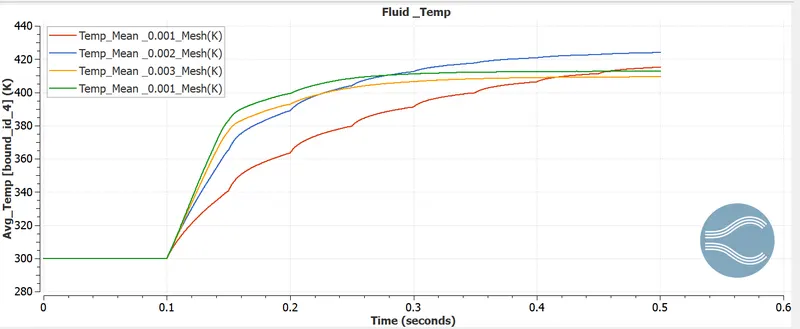
Fluid Side Temperature:

Mesh Size	Temperature
0.001	415
0.002	410
0.003	425
0.004	413

Solid_Temp:

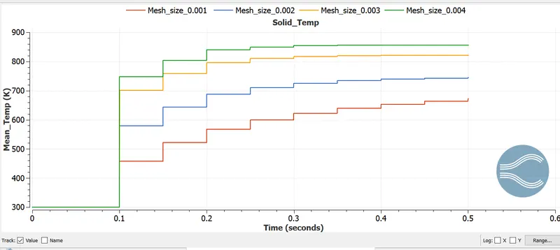
Solid Side temperature:

Mesh Size	Temperature
0.001	680
0.002	730
0.003	830
0.004	860

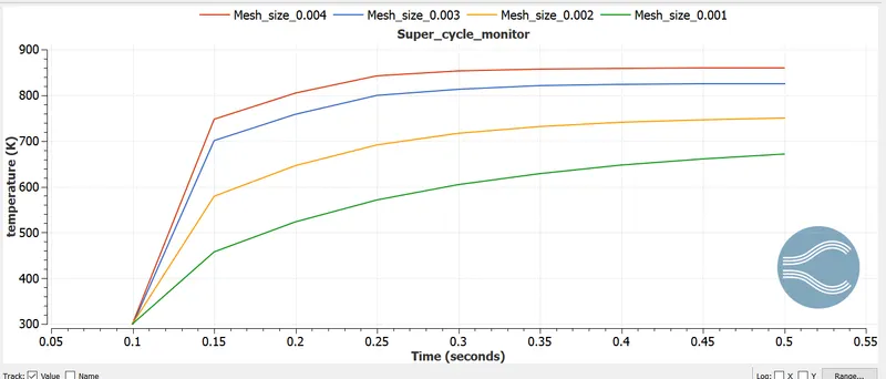
Super Cycle Monitor:

Mesh Size	Temperature
0.001	660
0.002	740
0.003	820
0.003	860

In this part we performed the grid dependency test with 0.001, 0.002,0.003,0.004 m Mesh size. By observing the above plots we can easily see that at the finer mesh we got the more accurate values of temperature, but at the finer mesh computational time has been increased .

The Super cyclic Interval are run by Mesh Size of 0.002 mm to be analyzed for a constant Mesh.

Intervals are 0.01, 0.02, 0.03

Case 1:0.01

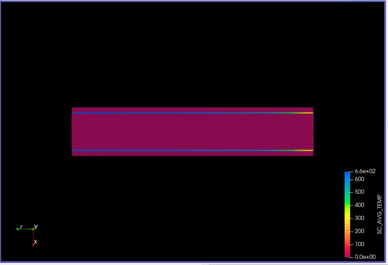
Super_cycling _Avg_Temp:

Super_cycling_HTC:

Super_cycling_Wall_Temp:

Case 2:0.02

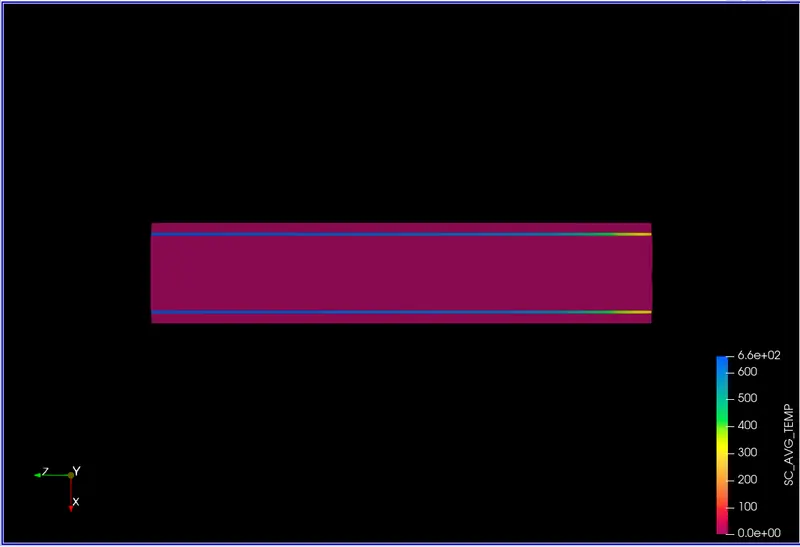
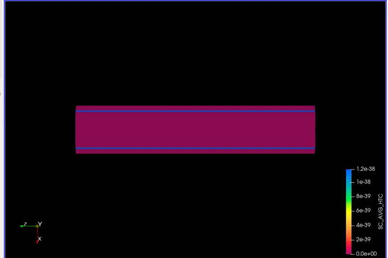
Super_cycling _Avg_Temp:

Super_cycling_HTC:

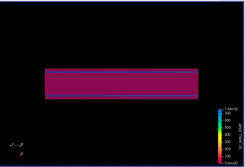
Super_cycling_Wall_Temp:

Case 3:0.03

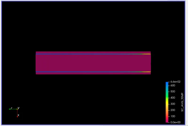
Super_cycling _Avg_Temp:

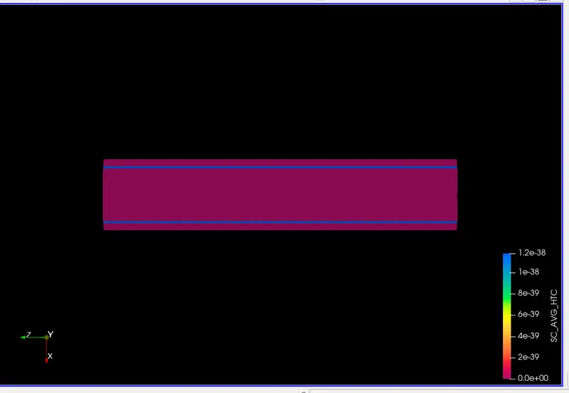
Super_cycling_HTC:

Super_cycling_Wall_Temp:

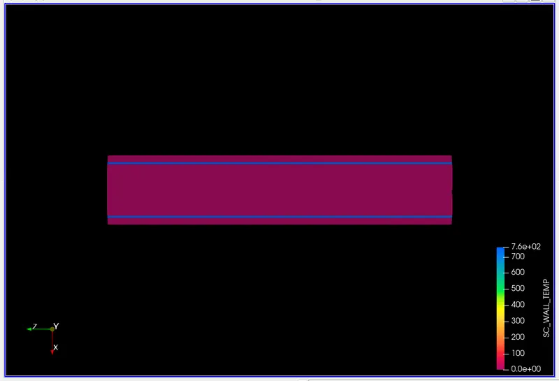
Super cyclic stage interval:

Fluid side main temperature:

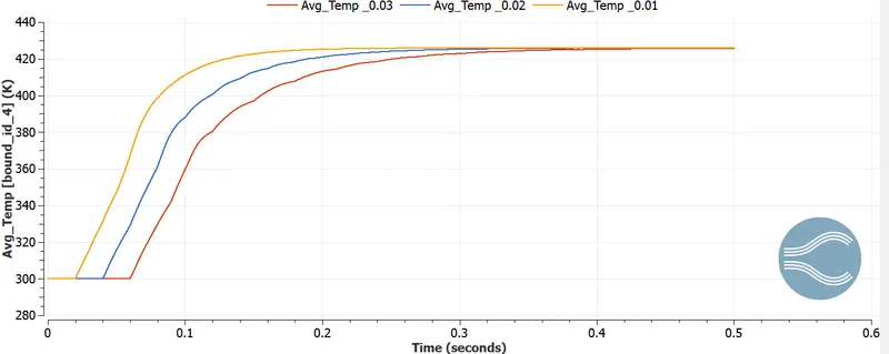
Super cyclic stage interval	Temperature
0.01	420
0.02	425
0.03	425

Solid side main temperature:

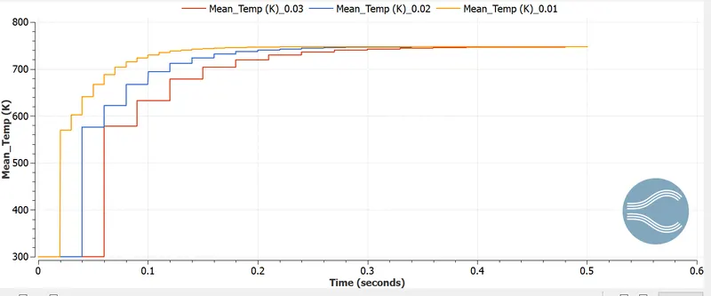
Super cyclic stage interval	Temperature
0.01	740
0.02	740
0.03	760

Super cycle at the monitor point:

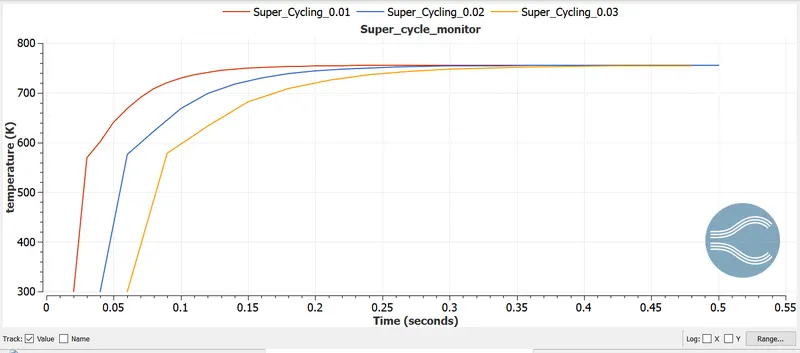
Super cyclic stage interval	Temperature
0.01	760
0.02	760
0.03	763

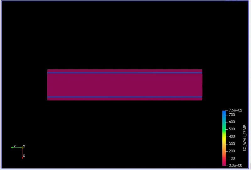
In the above results we can see the different values of super cycle stage interval. The time length for each stage from super cycling modelling is 0.01,0.02,0.03. In this super cycling mode converge continue to solve both the fluid and solid equations and store heat transfer coefficient and near the wall fluid cell temperature for a time equal to the super cycle stage interval.In the converge solves both fluid and solid equations together using the transient solver. ( but does not store the solid heat transfer data) from the start of simulation until the super cyclic start time in order to develop the fluid flow field. At super cycle start time converge begins storing values for a heat transfer coefficient and near the wall temp for each cell at the solid/fluid interface , one value for each time step.

In the above plots , we can see that setting the lower value of super cycle stage interval converges to the exact values of temp , Basically we increase the value of supercycle stage interval from 0.01 to 0.03, we got the more exact values at 0.03 super cycle interval

Mesh Time observed:

Mesh size (m)	Time (s)
0.001	63549
0.002	3036
0.003	829
0.004	127

Conclusion:

Result discussion of mesh in-dependency:

In this challenge we have performed the CHT analysis in a solid pipe

We have performed the grid dependency test with 0.001,0.002,0.003,0.004 m

From the above plots we can clearly see that the mesh finer, the accuracy in the result increases, But when the mesh goes finer the computational cost has increased.

Mesh size	0.001	0.002	0.003	0.004
Fluid mean temp (k)	415	410	425	413
Solid mean temp (k)	680	730	830	860
Computational time used	63549	3036	829	127

As we summarized in the above table , as the mesh becomes finer we got the values which is near to the exact solution. At the 0.001mesh we can observe that it takes too much time as compared to the other ones.

Result Discussion of the effect of super cycling:

We set the super cycling stage interval, I.e time in length for each cycle from super cycling modelling is used 0.01, 0.02and 0.03, And for smaller value of super cycling the converge achieves faster . A monitor point is also creates in the solid thickness boundary to observe the effects of super cycling . the plot shows that the steady state solver solves in the solid region at fixed intervals of time. And the results are compared while in the transient solver computing the fluid flow is temporarily stopped. Super cycling as done as the heat flow in the solids when depicted by a transient solver , is time consuming , Hence it is better to apply steady-state analysis for the heat transfer through the solids while studying the behaviour of fluid through the pipe.

Temperature profile in the solid region:

As we seen above, the steady state solver is employed in the solid region resulting in the sudden increase in temp at various time intervals,This does not represent the actual temp flow in the solid and only the steady state temp,

Note :The increase in temp in the solid region is due to the heat flux added to the solid outer wall.

Temperature profile in the Fluid region:

The transient solver is used to simulate the flow in the fluid region and hence the actual increase in the temp is observed in the case. The increase in temp is due to the transfer of heat from solid to fluid