Week 3.5 - Deriving 4th order approximation of a 2nd order derivative using Taylor Table method
Aim: To derive and write a program for fourth order approximation from second order derivative by following methods
1.central difference
2.skewed right sided difference
3.skewed left side difference
Objective:
1.To evaluate the second order derivative of the function ƒ(x) =exp(x)cosx,using above mentioned order of approximation
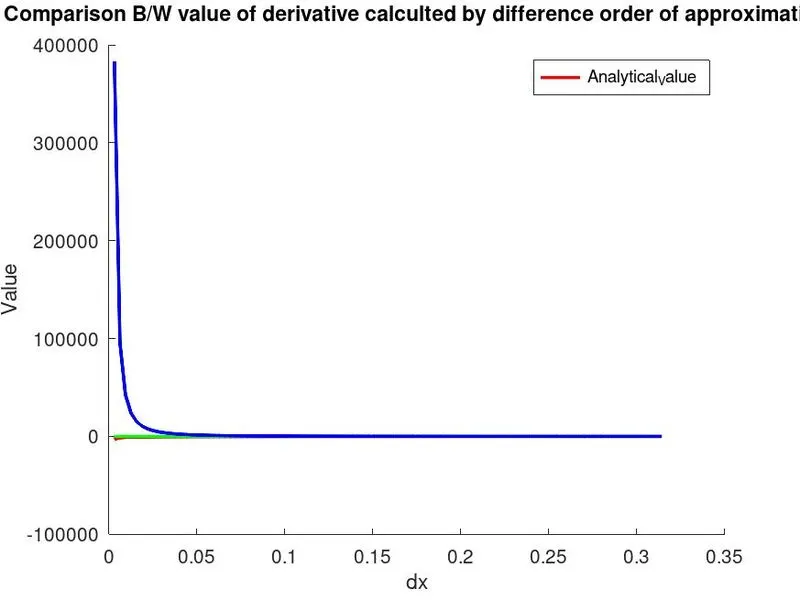
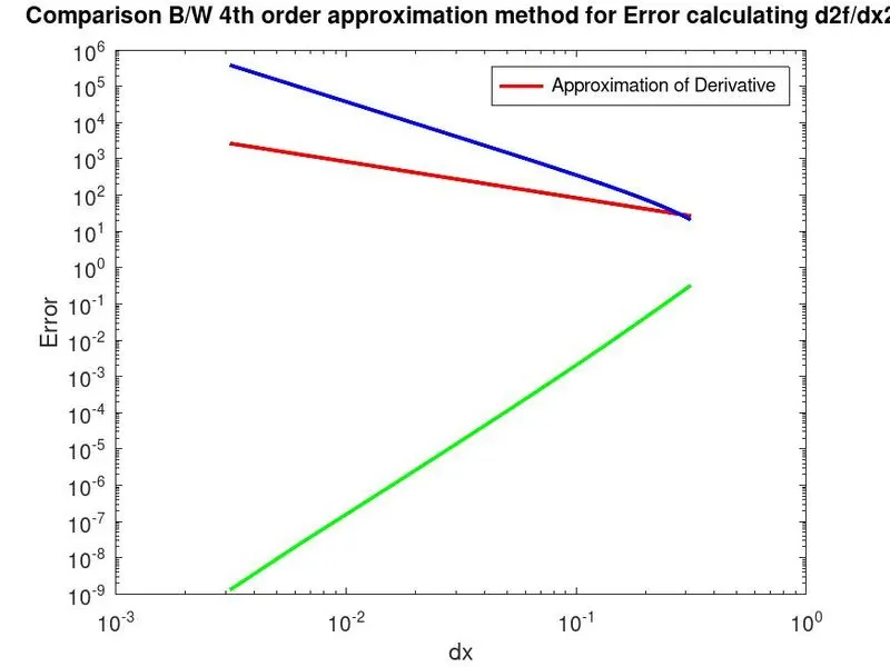
2. To plot and compare the values and errors of the 3 methods derived.
Theory and derivations:
During solving a CFD problem we may come across partial derivate equation which consists 2nd order derivative .since due to complexity of the equation ,we have to solve numerical approach rather than the analytical method,But when dealing with numerical approach we try to make the error margin as low as possible
As the order of approximation get higher ,we get high accuracy ,Hence ,We are going to derive the three methods of approximation for an analytical function.
The methods are following
1. Central difference: Hence the nodes selected are symmetrical I.e the data is taken from both sides of point of focus .using taylor’s method ,we get
Equation
`(del^2f)/(delx^2) =af(i-2)+bf(i-1)+cf(i)+df(i+1)+ef(i)`
Here there are two nodes taken from both side of the point of focus I.e . f(i).
(NOTE: To select the number of nodes in consideration,weuse following expression
N=p+q-1 for Central differencing
N=p+q for skewed differencing
Here N is no of nodes ,p is order of derivative and q is order of approximation
Taylor table for central difference:
|
f(x) |
dxf’(x) |
dx²f’’(x) |
dx³f’’’(x) |
dx⁴f’’’’(x) |
dx⁵f’’’’’(x) |
|
|
af(i-1) |
a |
-2a |
4a/2 |
-8a/6 |
16a/24 |
-32a/120 |
|
bf(i-2) |
b |
-b |
b/2 |
-b/6 |
b/24 |
-b/120 |
|
cf(1) |
c |
0 |
0 |
0 |
0 |
0 |
|
df(i+1) |
d |
d |
d/2 |
d/6 |
d/24 |
d/120 |
|
ef(i+2) |
e |
2e |
4e/2 |
8e/6 |
16e/24 |
32e/120 |
|
af(i-2)+bf(i-1)+cf(i)+df(i+1)+ef(i+2)` |
0 |
0 |
1 |
0 |
0 |
? |
This table transforms into matrix of type AX=B
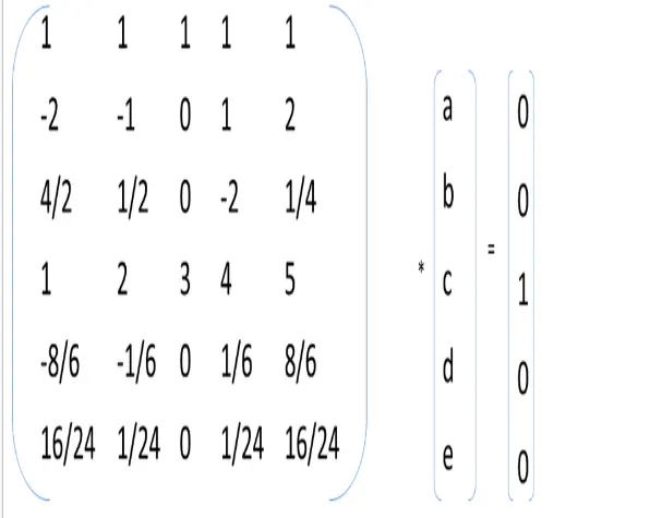
On further solving we get the values of the unknown i.e Values a=-0.0833 b=1.3333 c=-2.5000 d=1.3333 e=-0.0833
These coefficients will further used in code to get the values of derivative:
1.Skewed right hand side differencing : when the data point of the left nodes are not available (at initial boundary conditions ) then we have to relay on the available data set
`(del^2f)/(delx^2) =af(i)+bf(i+1)+cf(i+2)+df(i+3)+ef(i+4)+ff(i+5)`
Taylor table for Skewed right hand side differencing:
|
f(x) |
dxf’(x) |
dx²f’’(x) |
dx³f’’’(x) |
dx⁴f’’’’(x) |
dx⁵f’’’’’(x) |
|
|
af(i) |
a |
0 |
0 |
0 |
0 |
0 |
|
bf(i+1) |
b |
b |
b/2 |
b/6 |
b/24 |
b/120 |
|
cf(i+2) |
c |
2c |
4c/2 |
8c/6 |
16c/24 |
32/120 |
|
df(i+3) |
d |
3d |
9d/2 |
27d/6 |
81d/24 |
243d/120 |
|
ef(i+4) |
e |
4e |
16e/2 |
64e/6 |
256e/24 |
1024e/120 |
|
ff(i+5) |
f |
5f |
25f/2 |
125f/6 |
625f/24 |
3125f/120 |
|
af(i)+bf(i+1)+cf(i+2)+df(i+3)+ef(i+4)+ff(i+5)` |
0 |
0 |
1 |
0 |
0 |
0 |
This table transforms into matrix of type AX=B
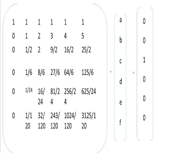
On further solving we get the values of the unknown i.e values = a=3.7500 b=-12.8333 c=17.8333 d=-13.0000 e=5.0833 f=-0.8333
These coefficients will further used in code to get the values of derivative:
1.Skewed left hand side differencing : when the data point of the right nodes are not available (at initial boundary conditions ) then we have to relay on the available data set
`(del^2f)/(delx^2) =af(i-5)+bf(i-4)+cf(i-3)+df(i-2)+ef(i-1)+ff(i)`
Taylor table for Skewed left hand side differencing:
|
f(x) |
dxf’(x) |
dx²f’’(x) |
dx³f’’’(x) |
dx⁴f’’’’(x) |
dx⁵f’’’’’(x) |
|
|
af(i-5) |
a |
-5a |
25a/2 |
-125a/6 |
625a/24 |
-3125a/120 |
|
bf(i-4) |
b |
-4b |
16b/2 |
-64b/6 |
256b/24 |
-1024b/120 |
|
cf(i-3) |
c |
-3c |
9c/2 |
-27c/6 |
81c/24 |
-243c/120 |
|
df(i-2) |
d |
-2d |
4d/2 |
-8d/6 |
16d/24 |
-32d/120 |
|
ef(i-1) |
e |
-e |
e/2 |
-e/6 |
-e/24 |
-e/120 |
|
ff(i) |
f |
0 |
0 |
0 |
0 |
0 |
|
af(i-5)+bf(i-4)+cf(i-3)+df(i-2)+ef(i-1)+ff(i)` |
0 |
0 |
1 |
0 |
0 |
0 |
This table transforms into matrix of type AX=B
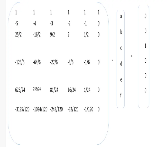
On further solving we get the values of the unknown i.e Values a=-0.0833 b= 5.0833 c=13.0000 d=17.8333 e=-12.8333 f=3.7500
Steps Involved:
1.We assign the value x and range of dx
2.We define an anonymous function of analytical function and its derivative
3.Use the matrices from above discussed section and solved it using inversion method i.e.
AX=B==>X=A^-1 B
And stored the coefficients in Cf1,cf2 and Cf3
4.Assigned the Rows and Coloumns to the appropriate matrices
5.Loop the order of approximation expression in a for loop under the range of dx.Hence here absolute error also calculated from the derivative value calculated analytically
6.The calculated values are plotted to do a better comparison
Result: