Week 6: Conjugate Heat Transfer Simulation
AIM
- Setup the CHT simulation flow through the pipe in converge CFD.
- Maintain the inlet Reynolds number as 7000
- Turn on the Y+ value before exporting all the setup files.
- Run grid dependence test by showing outlet temperatures are converging to a particular value.
- Find out the effect of supercycle stage interval by setting supercycle stage interval to 0.01,0.02and0.03.
- Compare the simulation time for the above three supercycle stage intervals.
Objective:
- To study of effect of super cycling on simulation
- Perform grid independency test for three different grid size
Introduction:
Conjugate heat transfer is coupled, fluid structurer, heat transfer where conduction heat transfer in solid wall interacts with fluid flow and convection heat transfer in fluid flow interacts with solid boundary
Steps
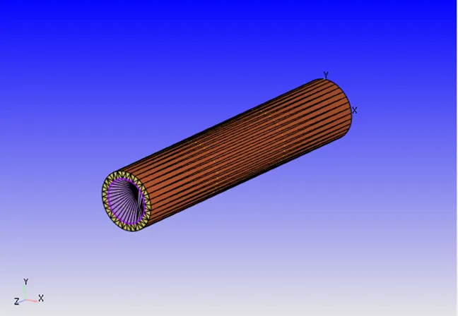
- First create geometry by one by taking following dimension
Inner Radius =0.015
Length=0.2
Outer Radius=0.02
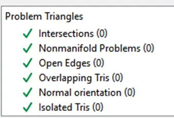
- Then check the diagnosis for any geometry error
- Setup the simulation
- Run the simulation in Cygwin
- Post process results in paraview
Geometry
Diagnosis
Calculation of inlet velocity:
Inlet Reynolds number =7000
Diameter of pipe=0.03 m
Dynamic viscosity of air=1.7894*10^-5
density=1.225 kg/m3
Re=rho*v*D/μ
v= (7000*1.7894*10^-5)/1.225*0.03
v=3.40 m/s
Case setup
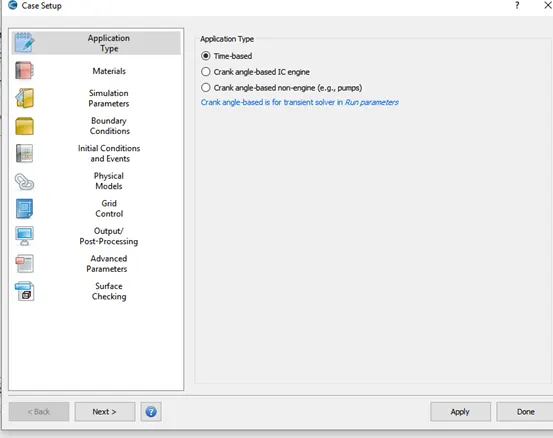
Applications-General flow (Time Based)
.
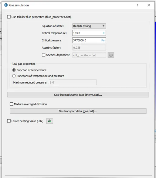
Gas Simulation:
Materials-
Gas: Air
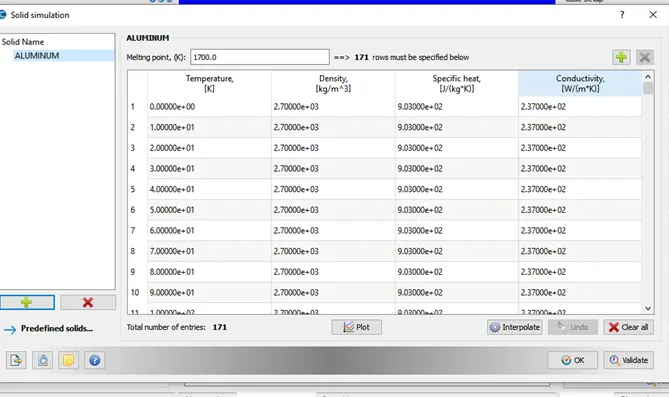
Solid: Aluminium
Solid Simulation
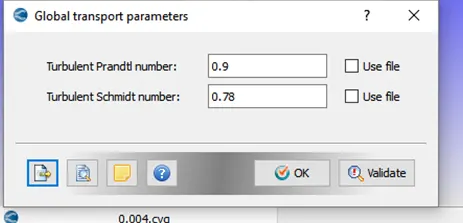
Global Transport parameters
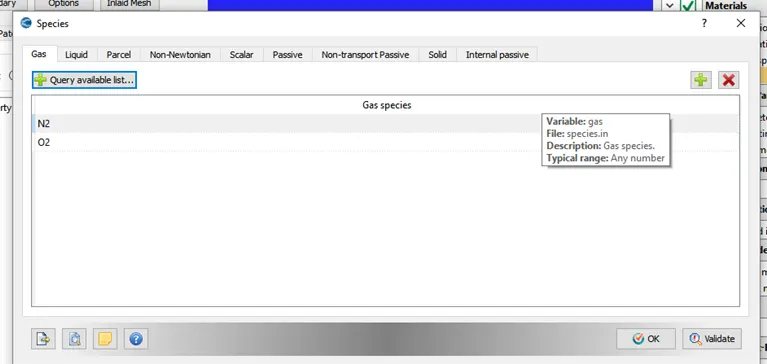
Species
Species-Gas-O2, N2
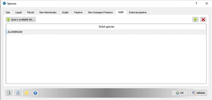
Solid- Aluminium
Run parameters:
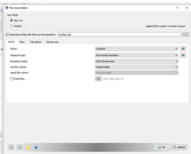
-Transient solver
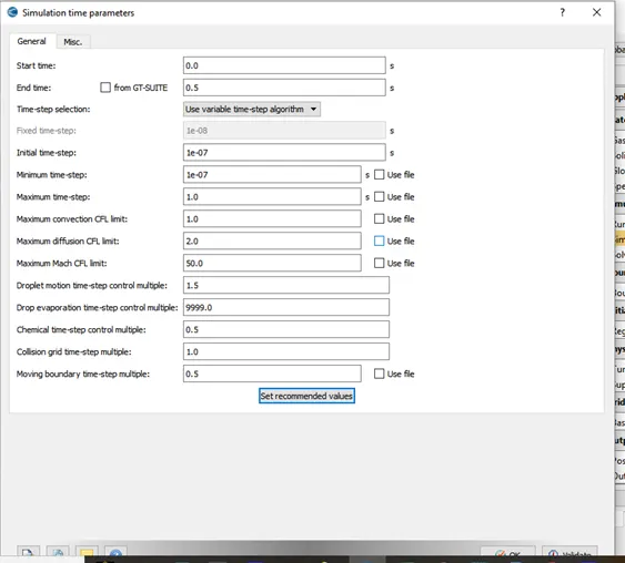
-Start time-0, End time-0.5 s
-Initial time step=minimum time step=1e-7 s
-Maximum time step=1 s
Simulation Time Parameters
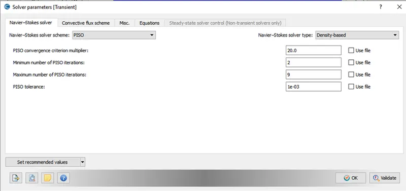
Density Based solver
Boundary conditions
Inlet- INFLOW-velocity-3.40 m/s
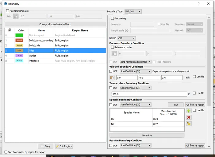
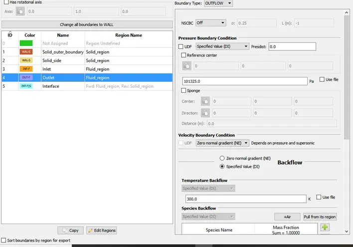
Outlet- OUTFLOW-Total pressure-101325 pa
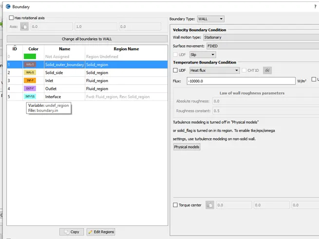
Solid outer wall- WALL, Heat flux= -10000 W/m2
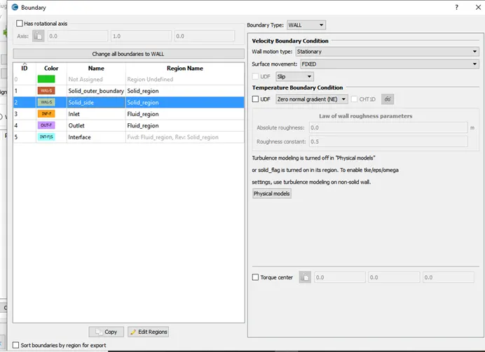
Solid wall -WALL velocity-slip , Temperature-zero normal gradient
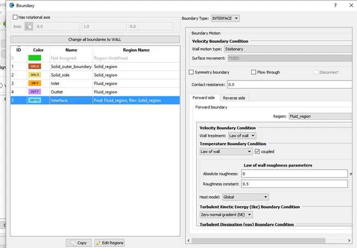
Interface- INTERFACE
Forward boundary-velocity and temperature-Law of wall ,region-fluid
Reverse boundary-velocity and temperature-slip and specified value ,region-solid
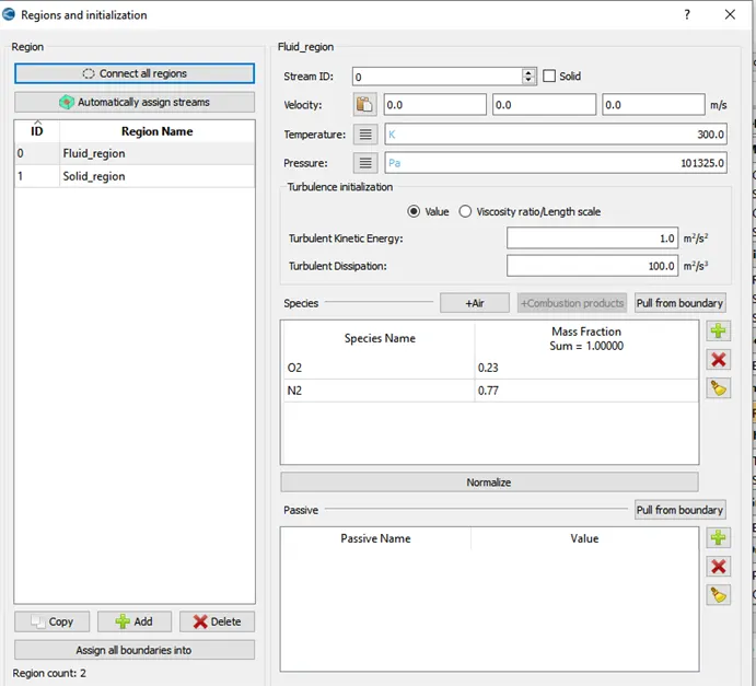
Region and initialization:
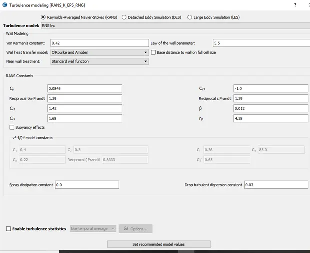
Turbulence Model
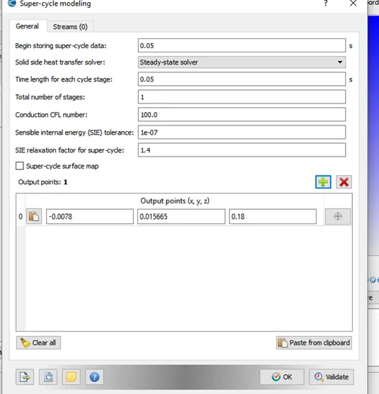
Super-Cycle Model
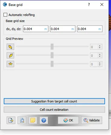
Base Grid
Results
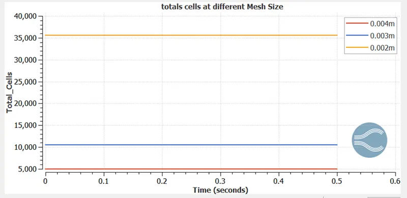
Totals cells
Total cells at different grid size
Grid Size Total cells (approximate)
0.004 m 5000
0.003 m 10000
0.002 m 35000
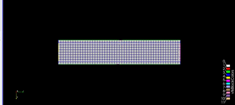
Grid size=0.004m
Mesh
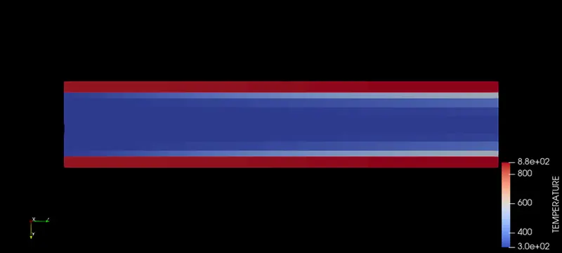
Temperature contour
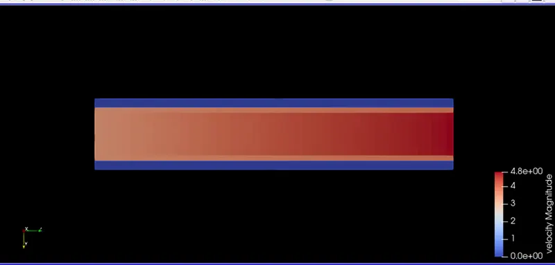
Velocity Contour
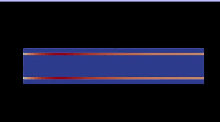
Y-plus
The maximum range is 15 for the mesh size 0.004m
Animation link
For Grid size:0.004m : https://youtu.be/FNwVrpy6Dxc
Case 2
Grid size=0.003m
Mesh

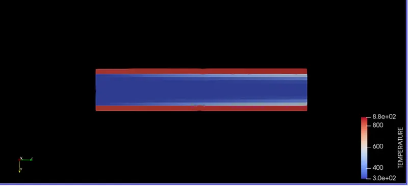
Temperature contour
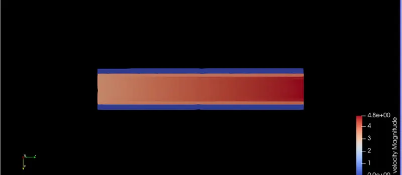
Velocity contour
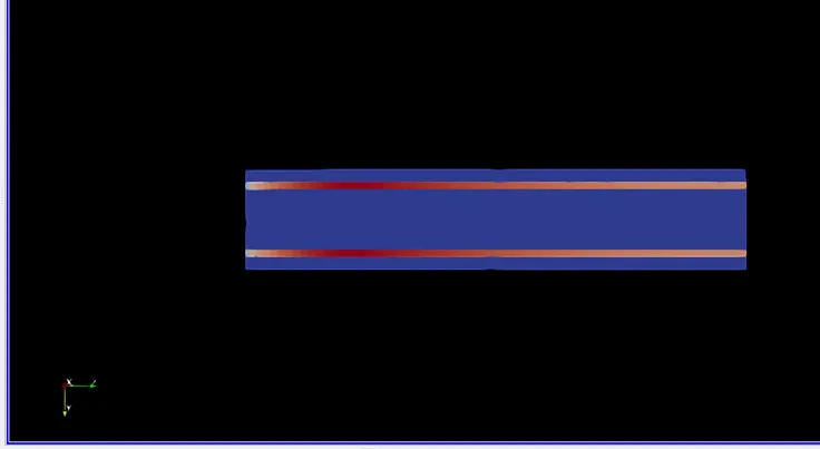
Y-plus
The maximum range is 13 for the mesh size 0.003m
Animation Link
For Grid size:0.003m : https://youtu.be/46y1ykL9UI0
Grid size=0.002m
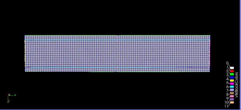
Mesh
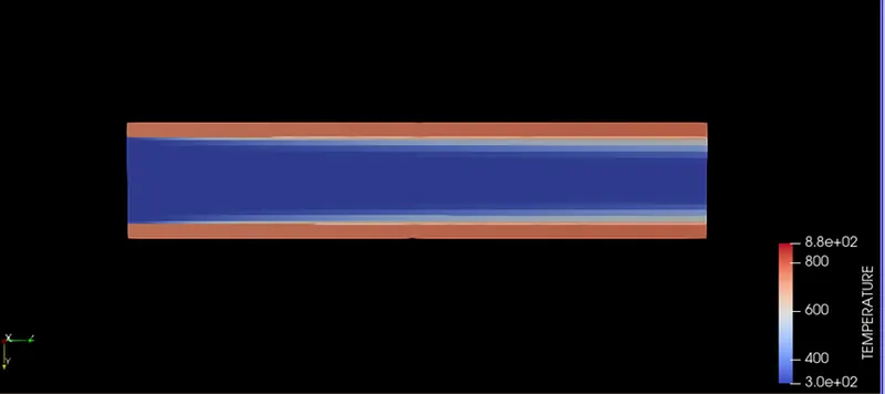
Temperature Contour
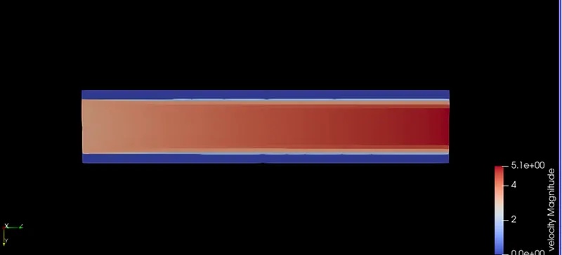
Velocity contour
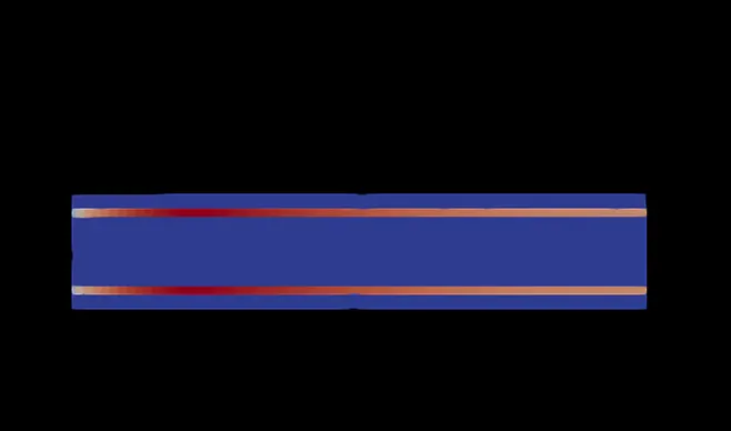
Y-plus
The maximum range is 10 for the mesh size 0.002m
Animation Link
For Grid size:0.002m : https://youtu.be/nNCCTRw9XKE
Mean temperature in fluid Region vs time:
The mean temperature for fluid region converged to around Approx 346 k for 0.004 m and approx 348 k for 0.003 m grid size. Whereas for 0.002m size the value is 360 K.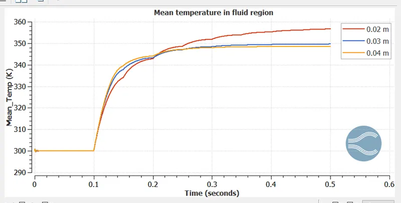
Mean temperature in Solid Region vs time:
The mean temperature for solid region converged to around 900 k for 0.004m grid size. Whereas for 0.003m and 0.002m size the value is 800 K and 750 k respectively.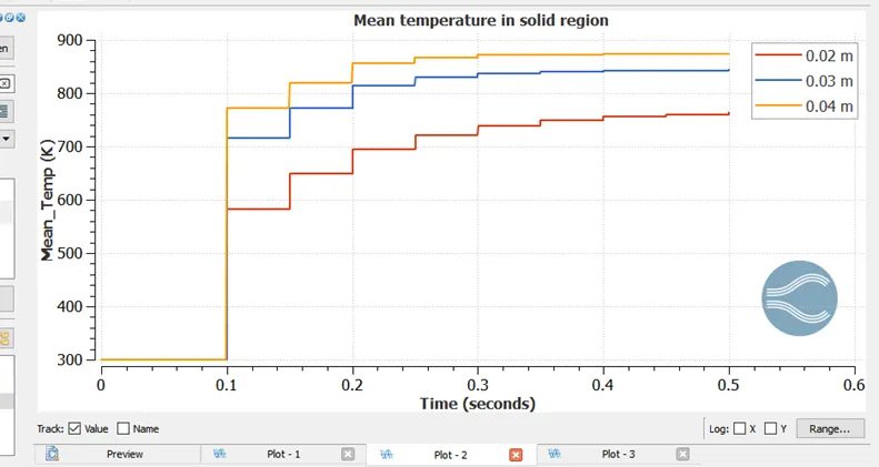
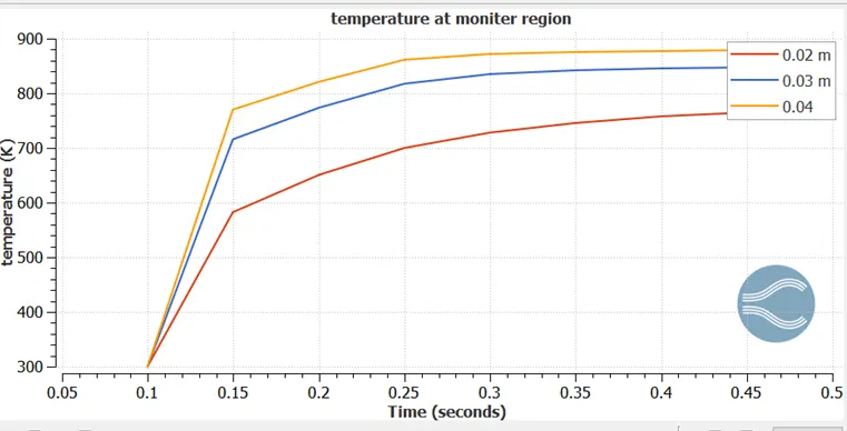
Mean temperature at monitor point vs time
The outlet temperature converged to around 850 k for 0.004m grid size. Whereas for 0.003m and 0.002m size the value is 820 K and 730 k respectively
Effect of super cycling stage interval
Super-cycling is a method used by CONVERGE in the case of conjugate heat transfer problems with a solid and liquid region. The solver for fluid and solid doesn’t run at same speed as heat transfer in fluid region is faster than solid region.
This causes problems during the solution given that the solid side solver would not have reached a steady state/convergence in the time the liquid solver does. This is where the concept of super-cycling can be used. Super-cycling is only meant to speed up the simulation
Three supercyle stage interval was set for comparison 0.01,0.02 and 0.03 respectively.
Mean temperature in fluid Region vs time:
The mean temperature for fluid region converged to around Approximate 345 k
We can see from the below graph that supercyle stage interval of 0.01 converged faster than stage interval with 0.02 and 0.03.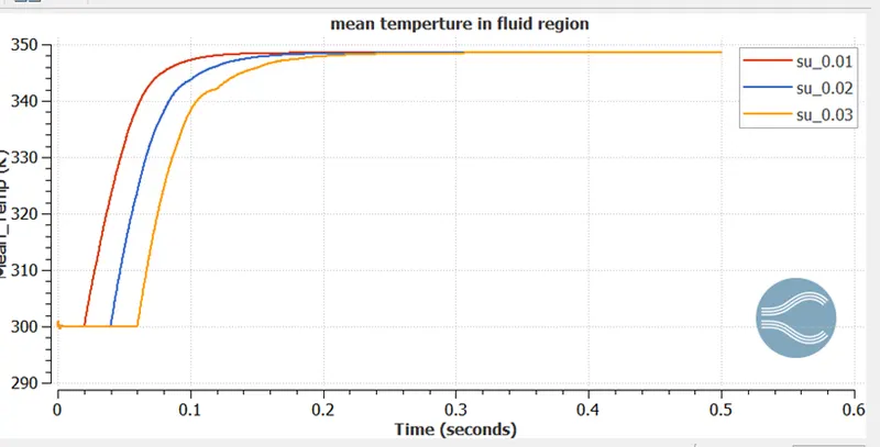
Mean temperature in Solid region Region vs time:
The mean temperature for solid region converged to around 850 k
We can see from the below graph that supercyle stage interval of 0.01 converged faster than stage interval with 0.02 and 0.03.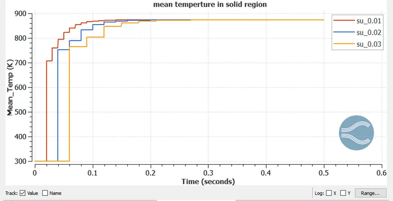
Mean temperature at monitor point vs time
The temperature at outlet monitor point converged to 850 k.
We can see from the below graph that supercyle stage interval of 0.01 converged faster than stage interval with 0.02 and 0.03.
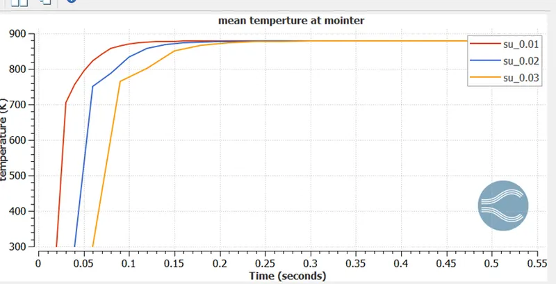
supercyle stage interval of 0.01 the convergence is the fastest in all the cases followed by 0.02 and 0.003 stage interval. So it can be concluded that lower value of super cycle stage interval gives faster convergence.
Time of simulation for different super cycle stage interval
| Super cycling Stage interval | Time of simulation |
| 0.03 | 977.10 s |
| 0.02 | 960.8 s |
| 0.01 | 899.1 s |
Animation:
For Grid size:0.004m:https://www.youtube.com/watch?v=lAGiflBl2C4
For Grid size:0.003m:https://www.youtube.com/watch?v=x26iVoaduwY
For Grid size:0.002m:https://www.youtube.com/watch?v=_mVmWHIC9q8
Conclusion
Conjugate heat transfer simulation for flow through a solid pipe was successfully performed.
- The grid dependency test showed that the temperature values approached a closed value when we decreased the mesh size and the solution was almost grid independent.
- supercyle stage interval of 0.01 the convergence is the fastest in all the cases followed by 0.02 and 0.003 stage interval. So, it can be concluded that lower value of super cycle stage interval gives faster convergence.