Project Report

CHT Analysis on a Graphics card

Introduction

Graphic Card or GPU is an electronic component often a computer's pepheral, responsible for computing the graphic signals, later transmitted to a graphic device. It has various range of performance as well as power usage. based on the design, the power rating is often specified on the package, the gpu may have a power rating of over 50W to 2000W. Many system architectures prefer modular gpu's for better power and accordingly heat management.

Objectives

The objective of present study is to simulate the cooling of graphic card, assisted by fins, which broadens the surface area and employs much beeter heat transfer.

The objective also includes calculating the heat transfer coefficient as well as maximum temperature attained by the processor in each case.

Outline of the Study

Conjugate heat transfer simulation has been done to achieve the objective. Since the study is of computational in nature, mesh refinement is a compulsory task. Mesh refinement strategy and study ahs been discussed in the next section. After mesh refinement the study has been followed up in three cases, as discussed below.

Case 1: -

Inlet Velocity of 1 m/s is to be applied at the inlet boundary.

Since the velocity is the least among all the cases, less cooling is expected in this case. Heat transfer coefficient and maximum temperature has to be calculated in this case.

Case 2: -

Inlet Velocity of 2 m/s is to be applied at inlet boundary.

Since there is slight increase in velocity as compared to previous case. The heat transfer coefficient and maximum temperature of the processor is expected to improve from the prior case.

Case 3: -

Inlet Velocity of 5m/s is to be applied at inlet boundary.

Since the velocity is increased further, the best performance among the three case is expected. Also, the velocity increase will lead to turbulent effect which can drastically affect the heat transfer. Altogether the best performance is expected in this case.

Mesh Refinement

In this study, heat transfer from the heat generating Unit (Processor) will get dissipated by 2 methods, conduction via fins and base plate and convection by air, since the effect of radiation has not been taken into account.

The geometries carrying the heat away from the processor are fins, base plate and vicinity fluid in these two media combined with fluid in contact with processor. Mesh refinement has been approached by changing the body sizing of these geometries.

Body size has been varied in 3 steps, at first, the elements of processor are decreased, succeeded by change in element size of fins then, the fluid body. Considering computational economy, the best model from each one has been applied to successive body sizing approach.

Surface Averaged Temperature has been assumed to be control variable for the mesh refinement study.

Refining the Processor Mesh

Element Size (m)	Value of Control variable
5e-4	195.94
4e-4	191.171
3e-4	193.715

There is a less variation in the control variable value with element size of 3e-4 and 4e-4 so mesh with less element size is used for the next refinement.

Refining the Fins Mesh

Element Size (m)	Value of Control variable
5e-4	171.16
4e-4	172.42
3.9e-4	170.29

Similarly, the element size of 4e-4 has been chosen as that of fin's.

Refining the Fluid Zone mesh

Element Size (m)	Value of Control variable
0.01	170.799
0.005	172.213

The element size of fluid zone is selected to be of 0.005m

Thus the size of element in processor is 0.0004m, 0.0004 of fin and 0.005 of fluid zone. The default mesh has been set to 0.005m. This would employ the base and other compoenents to be of that size accordingly.

Solution Methodology

After getting the element size ready for the simulation to have relatively optimum results, we proceed forward to create the full computational model.

Geometry

The geometry has been imported from the source and modified for computational formulation in Ansys – Space-Claim, Ansys geometry module.

ANsys Space-Claim has been used to prepare the model for further calculations.

At first the model files are checked for interferance, then the geometry is checked for overlaping, further the topology has been shared among the bodies.

The boundary names of the geometry has been presented below.

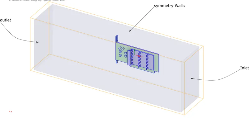
The walls of enclosure other than inlet and outlet are named as symmetry walls.

Meshing

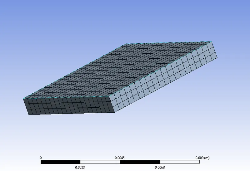
After geometry setup, the file is later used to create the computational mesh. As discussed in the mesh refinement section, appropriate element size has been used to create the mesh.

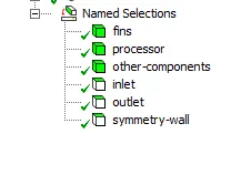
Appropriate named selection has been made to employ meshing as discribed below:

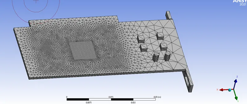
Final mesh of Processor

Final Mesh of Fins

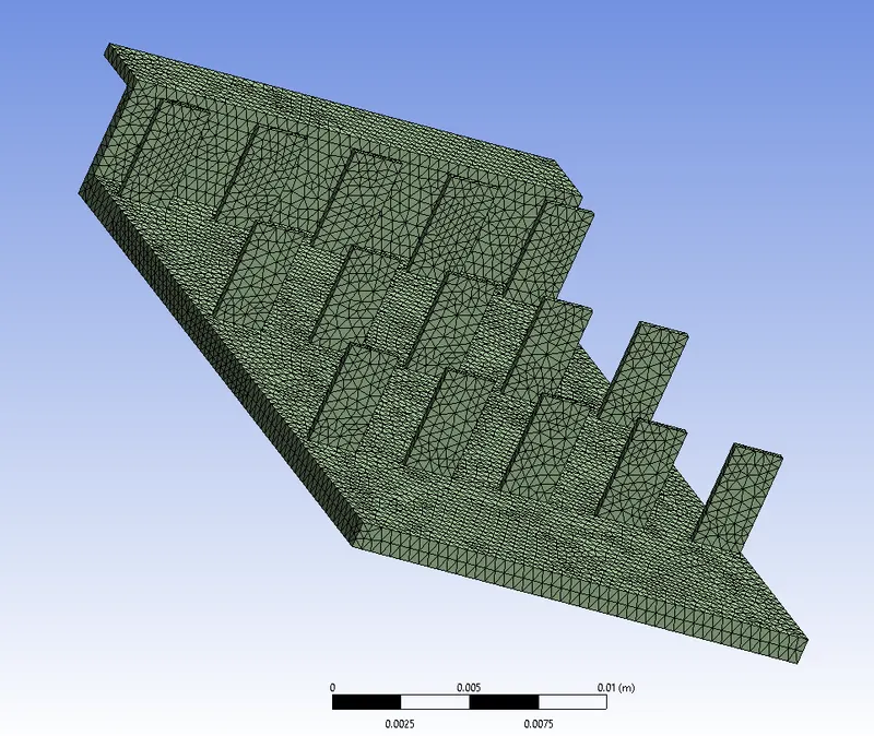
Final Mesh of Base and other components

Final Mesh of Fluid Zone

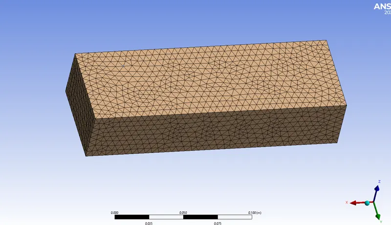
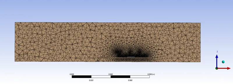
The complete Mesh of the computational domain

Element Quality Plot:

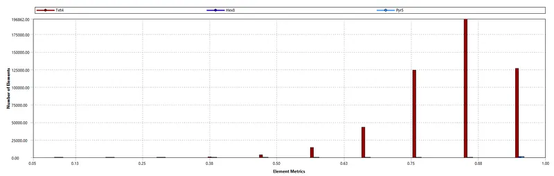
The final mesh is of total around 510K elements. The element quality plot is presented above. The mesh around the fins are denser than away from it. It is done to decrease the computational cost of the model all together.

Solver Settings

Later the mesh has been used to create the computational model.

Viscous Model

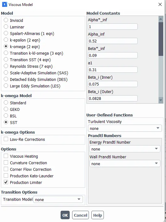
K – Omega -SST has been used as the viscous model. The turbulent effect will be predominant in the last case that is, with 5 m/s inlet velocity. The K-Omega SST has better wall as well as free stream performance also, the mesh has less no. of elements, so K-epsilon won’t be necessary in this case.

Material Modeling

Fins

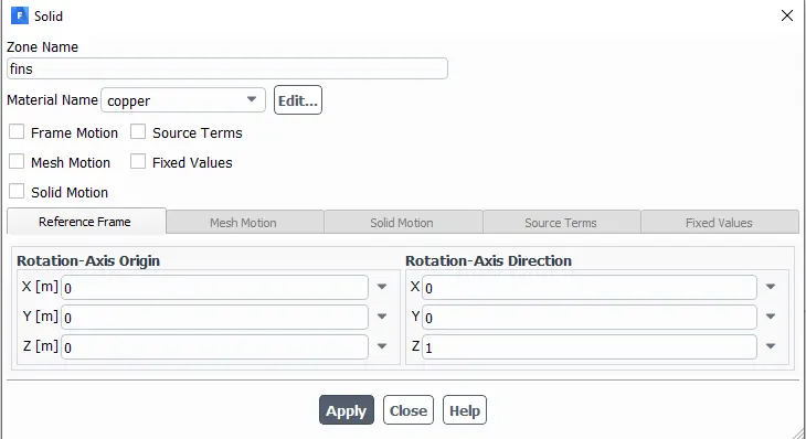
Copper is generally used as passive cooling media as it has high thermal conductivity and more stable at high temperature compared to aluminum.

Processor

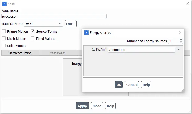
Processor package is enclosed under steel box, as it has high stability at elevated temperature. So, steel has been used for simulation of processor.

Base (Other-components)

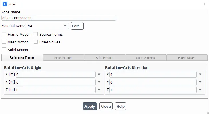
The base or remaining components are made up of substrate of different materials. It contains the entire circuit for connecting different components. FR4 has been choice of manufacturers for the product. Though it has low thermal conductivity, as its job is to maintain connection between intricate electronic items, that may be susceptible to high temperature. So, FR4 has been used to model the base components.

Boundary Conditions

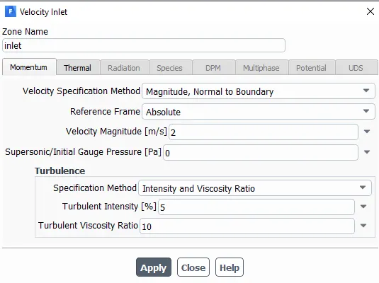
Inlet

Inlet is of velocity-inlet boundary, the value of velocity will be varied with the case being studied.

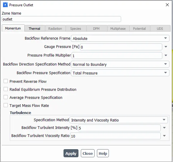
Outlet

Outlet is of pressure type boundary condition with 0-gauge pressure.

Heat Source

A constant heat source of 16W has been apploed to the processor zone. The heat source has been converted to volumentric heat source for its appplication. So, `{16}/{64mm^3}` = 250000000 `W/m^3`

Data Recording Setup

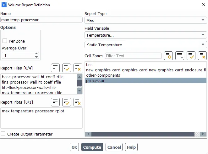
Maximum Processor Temperature

Volume maximum function in the Ansys solver module has been used to find out the maximum temperature attained by the processor.

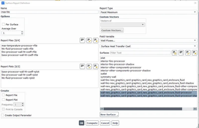
Maximum Heat Transfer Coefficient (Processor)

Facet maximum function in the Ansys solver module has been used to find out the maximum Heat Transfer Coefficient attained by the processor. The walls with fluid as has been chosen for the facet maximum to be calculated.

Results and Discussion

Simulating the developed computational model, the results ahs been described below

Case 1: -

Residual Plot

Contour Plot

Vector plot:

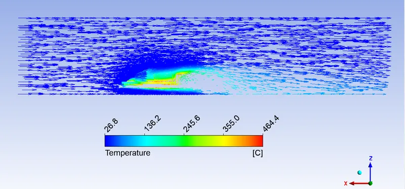
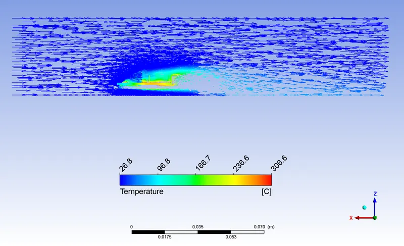
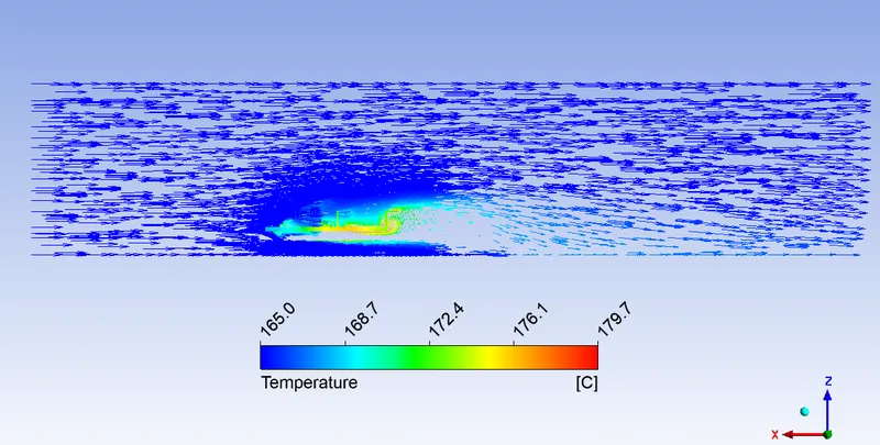
The vector represents the velocity, the color of the vector represents the temperature.

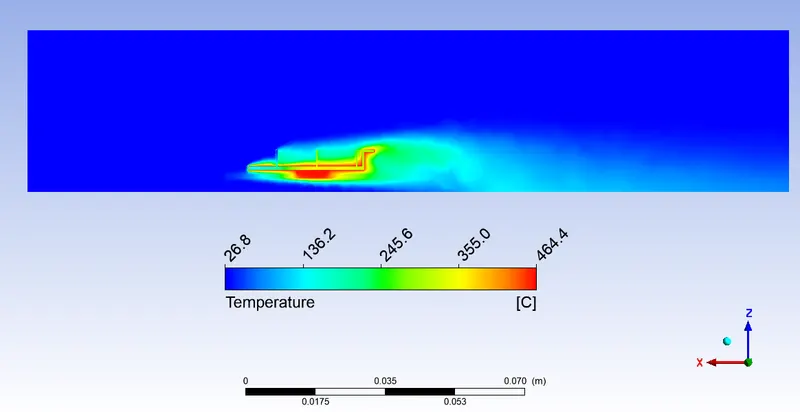
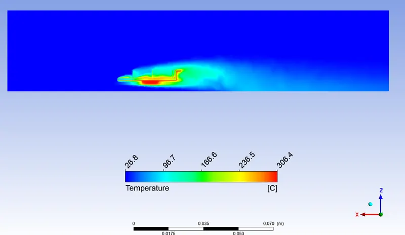
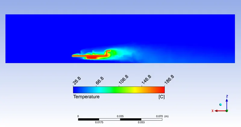
Color plot of temperature at lateral cross section clearly represnts the cooling of fins.

Case 2: -

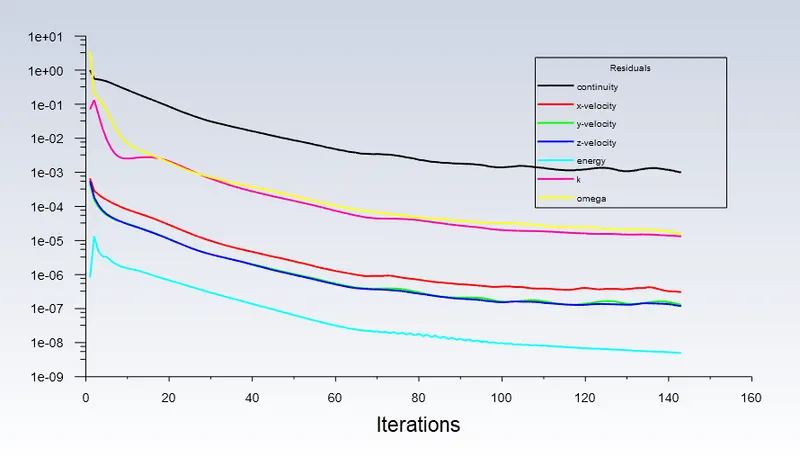
Residual Plot

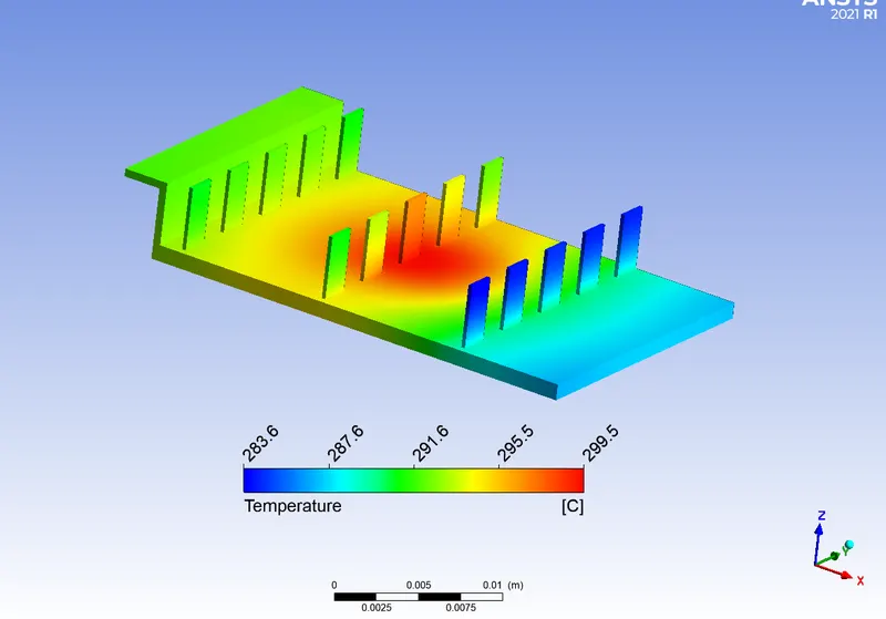
Contour plot

Vector Plot:

Color Plot:

Case 3: -

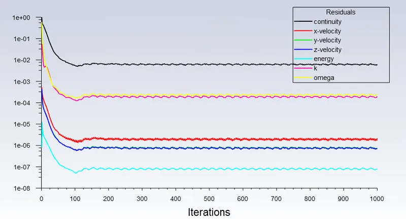
Residual Plot

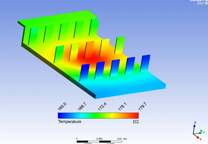
Contour Plot:

Vector Plot:

Color Plot:

Heat Transfer Coefficient of Fluid Processor Interface

Case	Heat Transfer Coefficient (W/m2K)
1	17.566
2	24.35
3	62.740

Maximum Temperature of Processor

Case	Temperature - Processor [C]
1	464.38
2	306.589
3	186.809

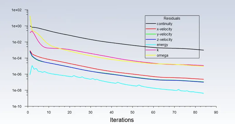
As seen from the presidual plots, it either goes below the tolerace range before no. of iteration or the residuals have near repeating pattern of iterations. This behaviour represents the converged solution.

As can be seen from the above table of heat transfer coefficient as well as Maximum temperature of the processor, as the velocity of inlet has increased, the cooling of processor has increased.

The fluid processor interface shows the similar trend, increase in velocity has lead to increase in cooling therefore, the heat transfer coefficient increases. This might have happened due to increase in velocity in the viscinity.

The model may be improved further by employing face sizing and having mesh refinement based on that. That would also increase the mesh density in the fluid region in the viscinity of the profile.